coords <- data.frame(
    name = c('T', 'C', 'P', 'U'),
    x =    c(1,    2,   0,  1),
    y =    c(1,    1,   1,  0)
)
dagify(
    T ~ P + C + U,
    P ~ U,
  coords = coords
) |> ggdag(seed = 2, layout = 'auto') + theme_dag()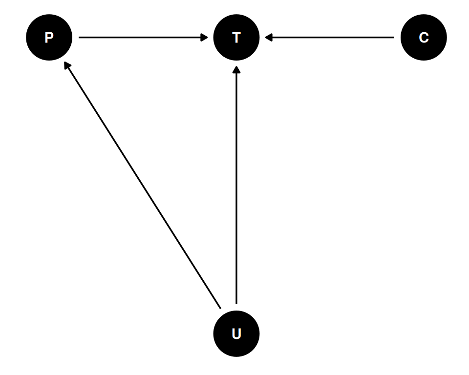
Gaussian process is “an infinite-dimensional generalization of multivariate normal distributions”. Instead of a conventional covariance matrix, use a kernel function that generalizes to infinite dimensions/observations/predictions. It allows you to use a smaller number of parameters, inside the covariance matrix, with regularization.
Given the kernel function, the covariance can get arbitrarily large because it doesn’t add any more parameters.
The kernel function can be based on differences, eg. space, time, age. These are continuous ordered categories. Partial pooling where points that are closer together to pool more.
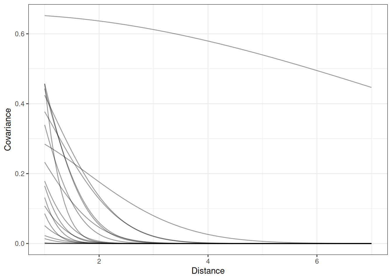
The kernel function describes the expected covariance between any two points separated by a given distance. The kernel function is estimated along with the other parameters.
Also see:
Goal is to describe the macro state, “what’s the shape of decline in covariation”. Some options:
Quadratic (L2)
Ornstein-Uhlenbeck
Periodic
Number of tool types associated with population size
Spatial covariation where islands close together share unobserved confounds and innovations. The effect of spatial covariation is to make closer islands have more similar tools or change in tools.
coords <- data.frame(
name = c('T', 'C', 'P', 'U'),
x = c(1, 2, 0, 1),
y = c(1, 1, 1, 0)
)
dagify(
T ~ P + C + U,
P ~ U,
coords = coords
) |> ggdag(seed = 2, layout = 'auto') + theme_dag()
Functional relationship
\[\Delta(T) = \alpha P^{\beta} - \gamma T\]
Statistical model
\[T_{i} \sim Poisson (\lambda_{i})\] \[\lambda_{i} = \hat{T}\] \[\hat{T} = \frac{\alpha P ^{\beta}}{\gamma}\]
Varying intercepts model
\[T_{i} \sim Poisson (\lambda_{i})\]
\[log \lambda_{i} = \bar{\alpha} + \alpha_{S_{[i]}}\] \[\hat{T} = \frac{\alpha P ^{\beta}}{\gamma}\]
\[\begin{bmatrix} \alpha_{1} \\ \alpha_{2} \\ .. \\ \alpha_{10} \end{bmatrix} \sim MVNormal(\begin{bmatrix} 0 \\ 0 \\ ... \\ 0 \end{bmatrix}, K)\] - vector of varying effects - vector of zeros - covariance matrix, a 10x10 kernel
Varying intercepts model
\[T_{i} \sim Poisson (\lambda_{i})\]
\[log \lambda_{i} = \bar{\alpha} + \alpha_{S_{[i]}}\] \[\begin{bmatrix} \alpha_{1} \\ \alpha_{2} \\ .. \\ \alpha_{10} \end{bmatrix} \sim MVNormal(\begin{bmatrix} 0 \\ 0 \\ ... \\ 0 \end{bmatrix}, K)\]
\[k_{i, j} = n^{2} exp(-\rho d^{2}_{i, j})\] - \(k_{i, j}\): covariance - \(n^{2}\): max covariance - \(\rho\): rate of decline - \(d^{2}_{i, j}\): distance i, j
\[\bar{\alpha} \sim Normal(3, 0.5)\] \[n^{2} \sim Exponential(2)\] \[\rho^{2} \sim Exponential(0.5)\]
\[T_{i} \sim Poisson (\lambda_{i})\] \[log \lambda_{i} = \frac{\bar{\alpha}P^{\beta}}{\gamma} exp(\alpha_{S_{[i]}})\] \[\begin{bmatrix} \alpha_{1} \\ \alpha_{2} \\ .. \\ \alpha_{10} \end{bmatrix} \sim MVNormal(\begin{bmatrix} 0 \\ 0 \\ ... \\ 0 \end{bmatrix}, K)\] \[k_{i, j} = n^{2} exp(-\rho d^{2}_{i, j})\] \[\bar{\alpha}, \beta, \gamma \sim Exponential(1)\] \[n^{2} \sim Exponential(2)\] \[\rho^{2} \sim Exponential(0.5)\]
Phylogenetic comparative methods are dominated by causal salad. Tossing factors into regression and interpreting every coefficient as causal. “Controlling for phylogeny” is often required by reviewers, papers often use AIC or cross validation criteria as a stand-in for causal inference.
Phylogenetic causation is a dynamical system where causation passes from one generation to the next, from the most recent ancestor to the subsequent time. The evolutionary history, however, is not known so the micro histories that may have happened have impacted the macro state, ie the pattern of covariation of living species. We want to model in a way that averages over the large number of possible histories.
Two conjoint problems:
Like social networks, phylogenies do not exist.
Different parts of the genome have different histories. Tree space is hard to explore statistically.
An evolutionary model and tree structure give us the pattern of covariation at the tips. Covariance declines with phylogenetic distance. The patttern of covariation at the tips can be used as a proxy for the unobserved confounds.
This requires an assumption about the covariance relationship with phylogenetic distance. Some options include the Ornstein-Uhlenbeck and Brownian motion.
Some next steps:
Data includes life history traits, eg. mass, brain volume, group size. Lots of missing data, measurement error and unobserved confounding.
coords <- data.frame(
    name = c('G', 'B', 'M', 'u', 'h'),
    x =    c(1,    3,   2,   2,   3),
    y =    c(1,    1,   0,   -1,  -1)
)
dagify(
    G ~ M + u,
    B ~ G + M + u,
    M ~ u,
    u ~ h,
  coords = coords
) |> ggdag(seed = 2, layout = 'auto') + theme_dag()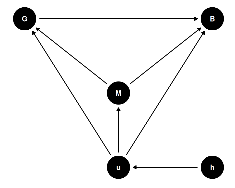
This is just one potential causal diagram. Reminder: there is no interpretation without causal representation.
\[B_{i} \sim Normal(\mu_{i}, \sigma)\] \[\mu_{i} = \alpha + \beta_{G} G_{i} + \beta_{M} M_{i}\] \[\alpha \sim Normal(0, 1)\] \[\beta_{G}, \beta_{M} \sim Normal(0, 0.5)\] \[\sigma \sim Exponential(1)\]
You can always re-express a linear regression of this type (a normal distribution assigned to each individual outcome, in this case \(B_{i}\)) with a multivariate normal distribution. This is an equivalent notation. The subscript i is taken off the outcome B, indicating they all come from some multivariate distribution with some mean \(\mu\) and covariance matrix \(K\).
\[B \sim MVNormal(\mu_{i}, K)\] \[\mu_{i} = \alpha + \beta_{G} G_{i} + \beta_{M} M_{i} + u_{i}\] \[K = I \sigma ^2\] - I is the identity matrix
\[\alpha \sim Normal(0, 1)\] \[\beta_{G}, \beta_{M} \sim Normal(0, 0.5)\] \[\sigma \sim Exponential(1)\]
\[B \sim MVNormal(\mu_{i}, K)\] \[\mu_{i} = \alpha + \beta_{G} G_{i} + \beta_{M} M_{i} + u_{i}\] \[K = n^2 exp(-\rho d_{i, j})\] - I is the identity matrix
\[\alpha \sim Normal(0, 1)\] \[\beta_{G}, \beta_{M} \sim Normal(0, 0.5)\] \[n^2 \sim HalfNormal(1, 0.25)\] - \(n^2\) is the maximum covariance prior
\[\rho \sim HalfNormal(3, 0.25)\]