targets::tar_source('R')Homework 06
Setup
Question 1
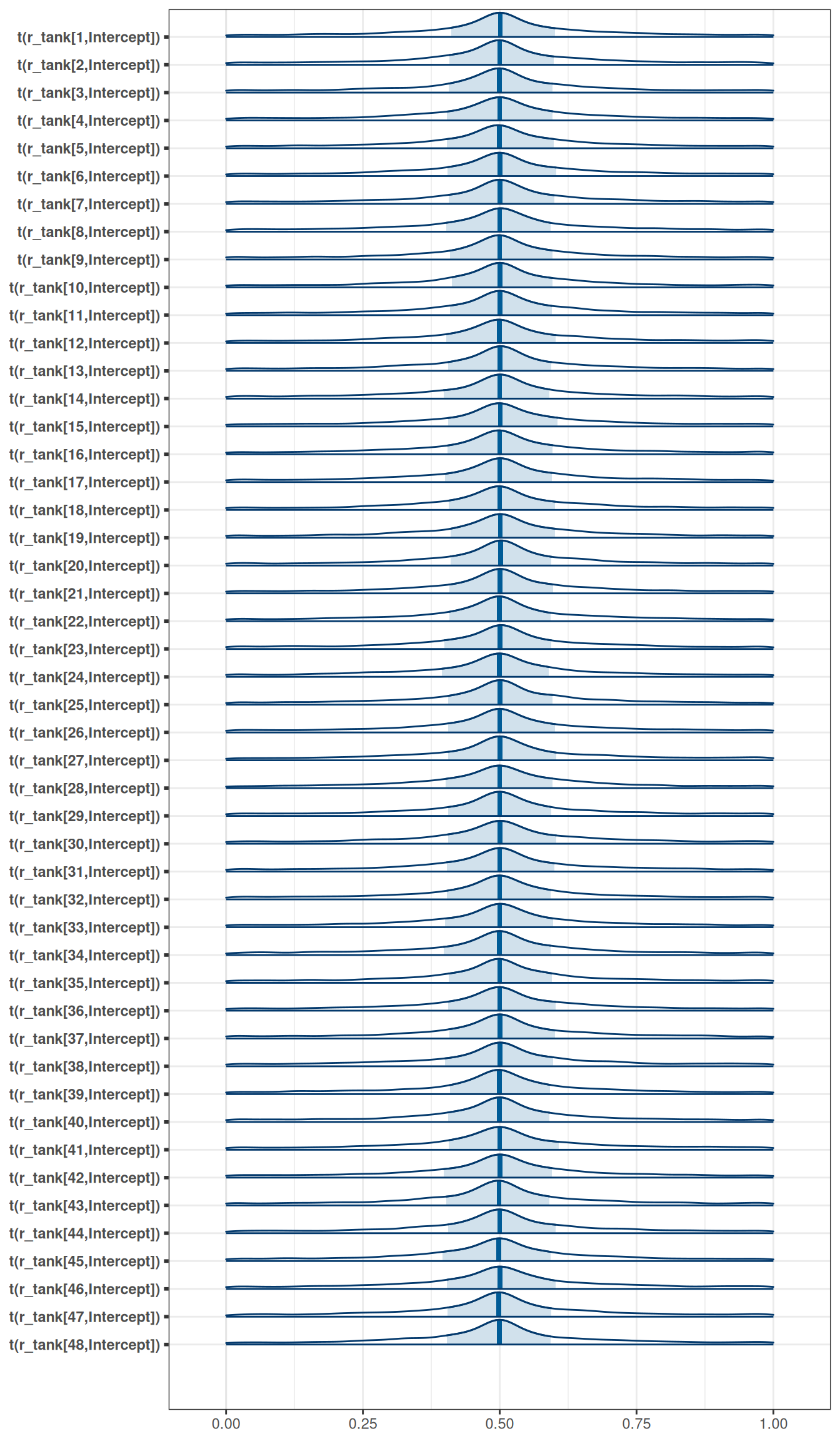
Conduct a prior predictive simulation for the Reedfrog model. By this I mean to simulate the prior distribution of tank survival probabilities. Start by using this prior:
\[\alpha_{j} \sim Normal(\bar{\alpha}, \sigma)\] \[\bar{\alpha} \sim Normal(0, 1)\] \[\sigma \sim Exponential(1)\]
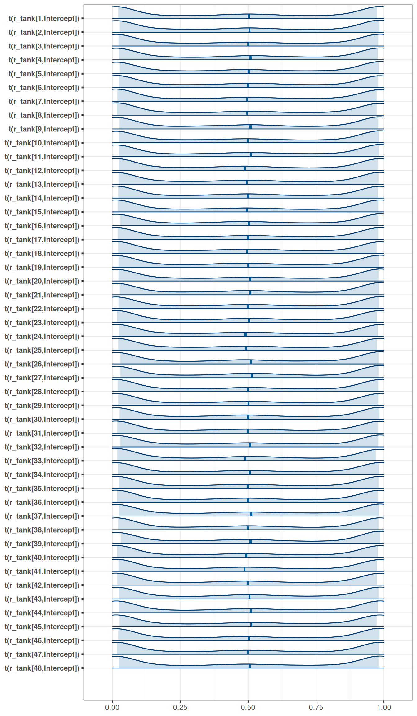
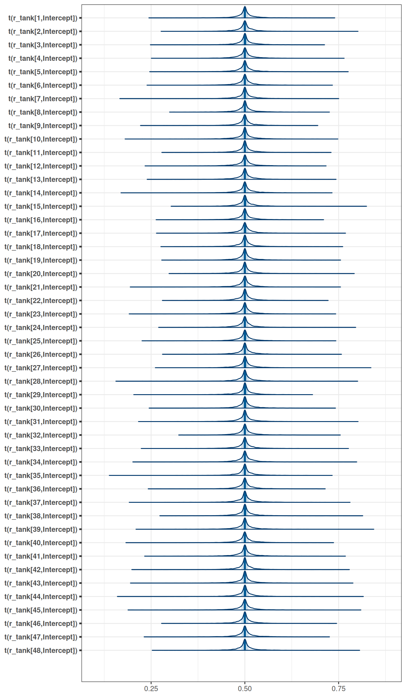
Be sure to transform the alpha j values to the probability scale for plotting and summary. How does increasing the width of the prior on sigma change the prior distribution of alpha j? You might try Exponential(10) and Exponential(0.1) for example.
Prior predictive simulation
# Load data
tar_load(reedfrogs)tar_load(h06_q01_exp_1_brms_sample_prior)
h06_q01_exp_1_brms_sample_prior$prior prior class coef group resp dpar nlpar lb ub source
normal(0, 1) Intercept user
exponential(1) sd 0 user
exponential(1) sd tank 0 (vectorized)
exponential(1) sd Intercept tank 0 (vectorized)mcmc_areas(
h06_q01_exp_1_brms_sample_prior,
regex_pars = 'r_tank',
transformations = inv_logit
)
tar_load(h06_q01_exp_0pt1_brms_sample_prior)
h06_q01_exp_0pt1_brms_sample_prior$prior
prior class coef group resp dpar nlpar lb ub source
normal(0, 1) Intercept user
exponential(0.1) sd 0 user
exponential(0.1) sd tank 0 (vectorized)
exponential(0.1) sd Intercept tank 0 (vectorized)mcmc_areas(
h06_q01_exp_0pt1_brms_sample_prior,
regex_pars = 'r_tank',
transformations = inv_logit
)
tar_load(h06_q01_exp_10_brms_sample_prior)
h06_q01_exp_10_brms_sample_prior$prior
prior class coef group resp dpar nlpar lb ub source
normal(0, 1) Intercept user
exponential(10) sd 0 user
exponential(10) sd tank 0 (vectorized)
exponential(10) sd Intercept tank 0 (vectorized)mcmc_areas(
h06_q01_exp_10_brms_sample_prior,
regex_pars = 'r_tank',
transformations = inv_logit
)
Question 2
Revisit the Reedfrog survival data, data(reedfrogs). Start with the varying effects model from the book and lecture. Then modify it to estimate the causal effects of the treatment variables pred and size, including how size might modify the effect of predation. An easy approach is to estimate an effect for each combination of pred and size. Justify your model with a DAG of this experiment
Estimand
What is the causal effect of predation and size on survival?
Scientific model
coords <- data.frame(
    name = c('D', 'G', 'P', 'T', 'S'),
    x =    c(1,    2,   3,   1,    2),
    y =    c(0,    0,   0,   1,  1)
)
dag <- dagify(
S ~ D + G + P + T,
coords = coords,
outcome = 'S',
exposure = c('G', 'P')
)
ggdag(dag, seed = 2, layout = 'auto') + theme_dag()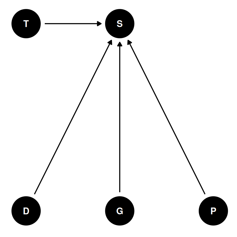
- 48 tanks (T) of reedfrogs
- treatments: density (D), size (G), predation (P)
- outcome: survival (S)
Adjustment set
ggdag_adjustment_set(dag, effect = 'direct') + theme_dag()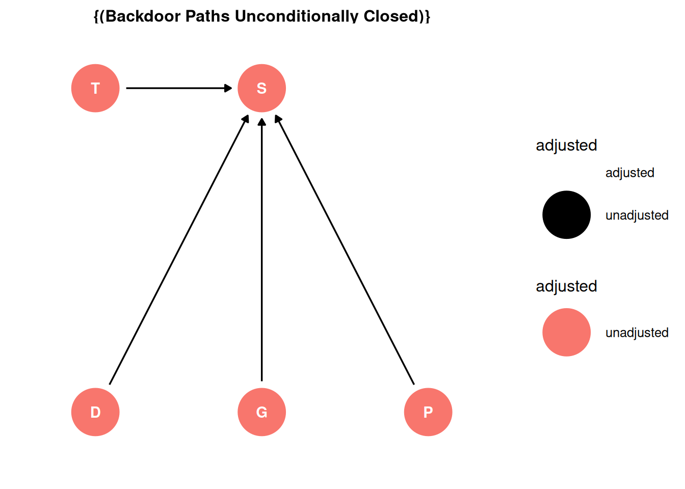
Analyze the data
# Load model
tar_load(h06_q02_brms_sample)
h06_q02_brms_sample
Family: binomial
Links: mu = logit
Formula: surv | trials(density) ~ 1 + pred * size + (1 | tank)
Data: h06_q02_brms_data (Number of observations: 48)
Draws: 4 chains, each with iter = 2000; warmup = 1000; thin = 1;
total post-warmup draws = 4000
Multilevel Hyperparameters:
~tank (Number of levels: 48)
Estimate Est.Error l-95% CI u-95% CI Rhat Bulk_ESS Tail_ESS
sd(Intercept) 0.60 0.11 0.39 0.84 1.00 2366 3084
Regression Coefficients:
Estimate Est.Error l-95% CI u-95% CI Rhat Bulk_ESS Tail_ESS
Intercept 2.42 0.26 1.92 2.95 1.00 3325 3205
predpred -2.74 0.32 -3.37 -2.09 1.00 2578 2881
sizesmall 0.16 0.35 -0.52 0.86 1.00 2709 3141
predpred:sizesmall 0.56 0.43 -0.31 1.40 1.00 2404 2819
Draws were sampled using sample(hmc). For each parameter, Bulk_ESS
and Tail_ESS are effective sample size measures, and Rhat is the potential
scale reduction factor on split chains (at convergence, Rhat = 1).# Estimated marginal effects
marg_eff <- emmeans(h06_q02_brms_sample, ~ size*pred, regrid = 'response')
marg_eff size pred prob lower.HPD upper.HPD
big no 0.918 0.876 0.953
small no 0.929 0.892 0.961
big pred 0.418 0.319 0.524
small pred 0.598 0.496 0.697
Point estimate displayed: median
HPD interval probability: 0.95 plot(marg_eff) + labs(x = 'Survival', y = 'Size : Predation')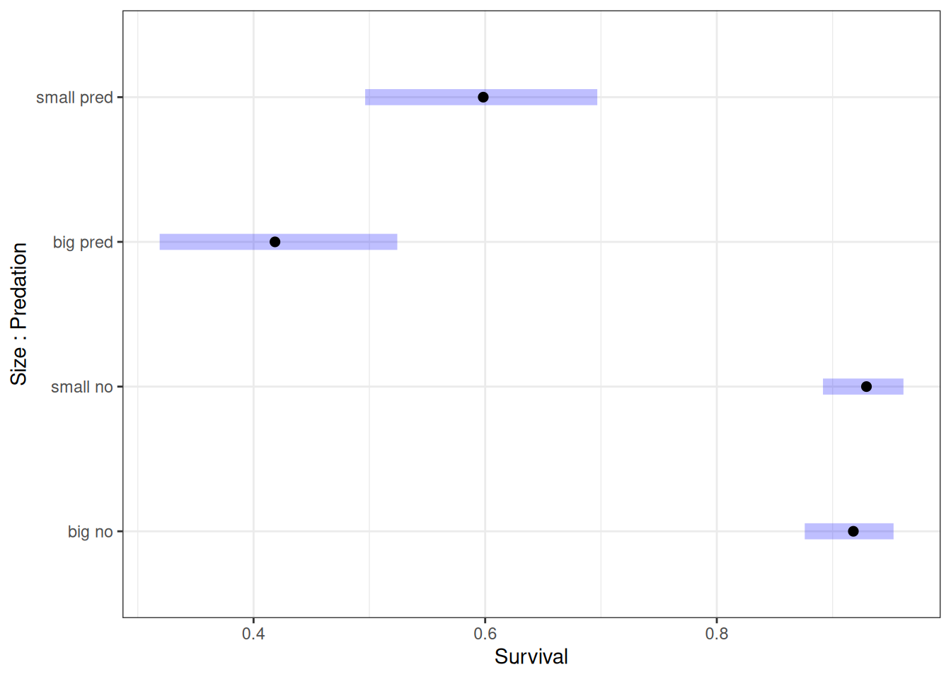
Question 3
3-OPTIONAL CHALLENGE. Return to the Trolley data, data(Trolley), from Chapter 12. Define and fit a varying intercepts model for these data. By this I mean to add an intercept parameter for the individual participants to the linear model. Cluster the varying intercepts on individual participants, as indicated by the unique values in the id variable. Include action, intention, and contact as treatment effects of interest. Compare the varying intercepts model and a model that ignores individuals. What is the impact of individual variation in these data?
Estimand
What is the causal effect of action, intention and contact on survey responses, considering the variation of individuals?
Scientific model
coords <- data.frame(
    name = c('X', 'R', 'S', 'E', 'Y', 'G',  'P'),
    x =    c(1,    2,   3,   1,    2,   3,  2),
    y =    c(0,    0,   0,   -2,  -1,  -2,  -3)
)

dag <- dagify(
    R ~ X + S + E + Y + G,
    E ~ Y + G,
  coords = coords
)
ggdag(dag, seed = 2, layout = 'auto') + theme_dag()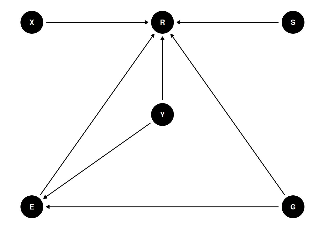
- R: response to the trolley story
- X: action, intention, contact
- S: story
- E: education
- Y: age
- G: gender
Analyze the data
tar_load(trolley)

tar_load(h06_q03_no_ind_var_brms_sample)
tar_load(h06_q03_ind_var_brms_sample)

h06_q03_no_ind_var_brms_sample
Family: cumulative
Links: mu = logit; disc = identity
Formula: response ~ action + intention + contact
Data: h06_q03_no_ind_var_brms_data (Number of observations: 9930)
Draws: 4 chains, each with iter = 2000; warmup = 1000; thin = 1;
total post-warmup draws = 4000
Regression Coefficients:
Estimate Est.Error l-95% CI u-95% CI Rhat Bulk_ESS Tail_ESS
Intercept[1] -2.83 0.05 -2.92 -2.74 1.00 2852 2513
Intercept[2] -2.15 0.04 -2.24 -2.07 1.00 3311 2649
Intercept[3] -1.57 0.04 -1.65 -1.49 1.00 3371 2981
Intercept[4] -0.55 0.04 -0.62 -0.48 1.00 3692 3232
Intercept[5] 0.12 0.04 0.05 0.19 1.00 3963 3357
Intercept[6] 1.02 0.04 0.95 1.10 1.00 4207 3415
action -0.71 0.04 -0.79 -0.62 1.00 3790 2873
intention -0.72 0.04 -0.79 -0.65 1.00 4356 3247
contact -0.96 0.05 -1.06 -0.86 1.00 4065 2910
Further Distributional Parameters:
Estimate Est.Error l-95% CI u-95% CI Rhat Bulk_ESS Tail_ESS
disc 1.00 0.00 1.00 1.00 NA NA NA
Draws were sampled using sample(hmc). For each parameter, Bulk_ESS
and Tail_ESS are effective sample size measures, and Rhat is the potential
scale reduction factor on split chains (at convergence, Rhat = 1).h06_q03_ind_var_brms_sample Family: cumulative
Links: mu = logit; disc = identity
Formula: response ~ action + intention + contact + (1 | id)
Data: h06_q03_ind_var_brms_data (Number of observations: 9930)
Draws: 4 chains, each with iter = 2000; warmup = 1000; thin = 1;
total post-warmup draws = 4000
Multilevel Hyperparameters:
~id (Number of levels: 331)
Estimate Est.Error l-95% CI u-95% CI Rhat Bulk_ESS Tail_ESS
sd(Intercept) 1.89 0.08 1.73 2.05 1.00 654 1167
Regression Coefficients:
Estimate Est.Error l-95% CI u-95% CI Rhat Bulk_ESS Tail_ESS
Intercept[1] -3.95 0.12 -4.17 -3.73 1.01 373 838
Intercept[2] -3.03 0.11 -3.25 -2.82 1.01 354 742
Intercept[3] -2.25 0.11 -2.46 -2.03 1.01 345 737
Intercept[4] -0.78 0.11 -0.99 -0.57 1.01 336 754
Intercept[5] 0.26 0.11 0.04 0.47 1.01 334 838
Intercept[6] 1.66 0.11 1.44 1.88 1.01 357 825
action -0.96 0.04 -1.04 -0.87 1.00 6949 3184
intention -0.95 0.04 -1.03 -0.88 1.00 7202 3024
contact -1.27 0.05 -1.38 -1.17 1.00 6878 3113
Further Distributional Parameters:
Estimate Est.Error l-95% CI u-95% CI Rhat Bulk_ESS Tail_ESS
disc 1.00 0.00 1.00 1.00 NA NA NA
Draws were sampled using sample(hmc). For each parameter, Bulk_ESS
and Tail_ESS are effective sample size measures, and Rhat is the potential
scale reduction factor on split chains (at convergence, Rhat = 1).tidy_selected_vars <- function(m, vars) {
draws <- tidy_draws(m) |>
gather_variables()
setDT(draws)
draws[.variable %in% vars]
}
sel_vars <- c('b_action', 'b_intention', 'b_contact')
no_ind_var <- tidy_selected_vars(h06_q03_no_ind_var_brms_sample, sel_vars)
no_ind_var[, type := 'No individual variation']
ind_var <- tidy_selected_vars(h06_q03_ind_var_brms_sample, sel_vars)
ind_var[, type := 'Varying intercepts for each individual']
ggplot(rbindlist(list(no_ind_var, ind_var))) +
stat_halfeye(position = 'dodge',
aes(inv_logit(.value),
type,
fill = type),
alpha = 0.2) +
guides(fill = 'none') +
labs(x = 'inv_logit(parameter estimate)', y = '') +
xlim(0, 1) +
facet_wrap(~.variable, ncol = 1)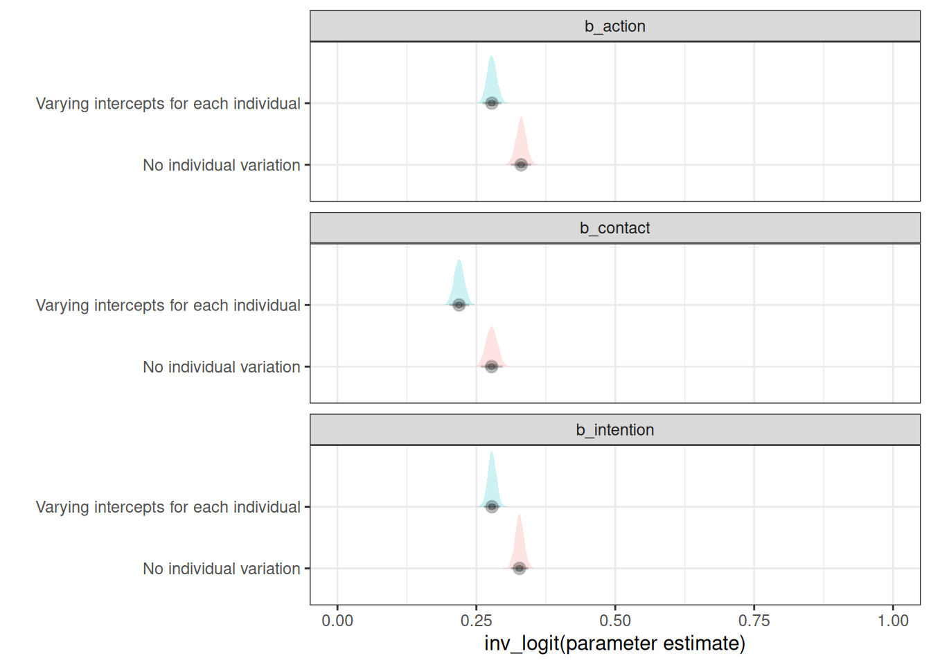
Parameter estimates for intention, action and contact for the model that includes varying intercepts for each individual are consistently lower than the model that ignores individual variation.