Homework 01

Setup

library(ggplot2)
source('R/globe_tossing.R')
theme_set(theme_bw())

Question 1

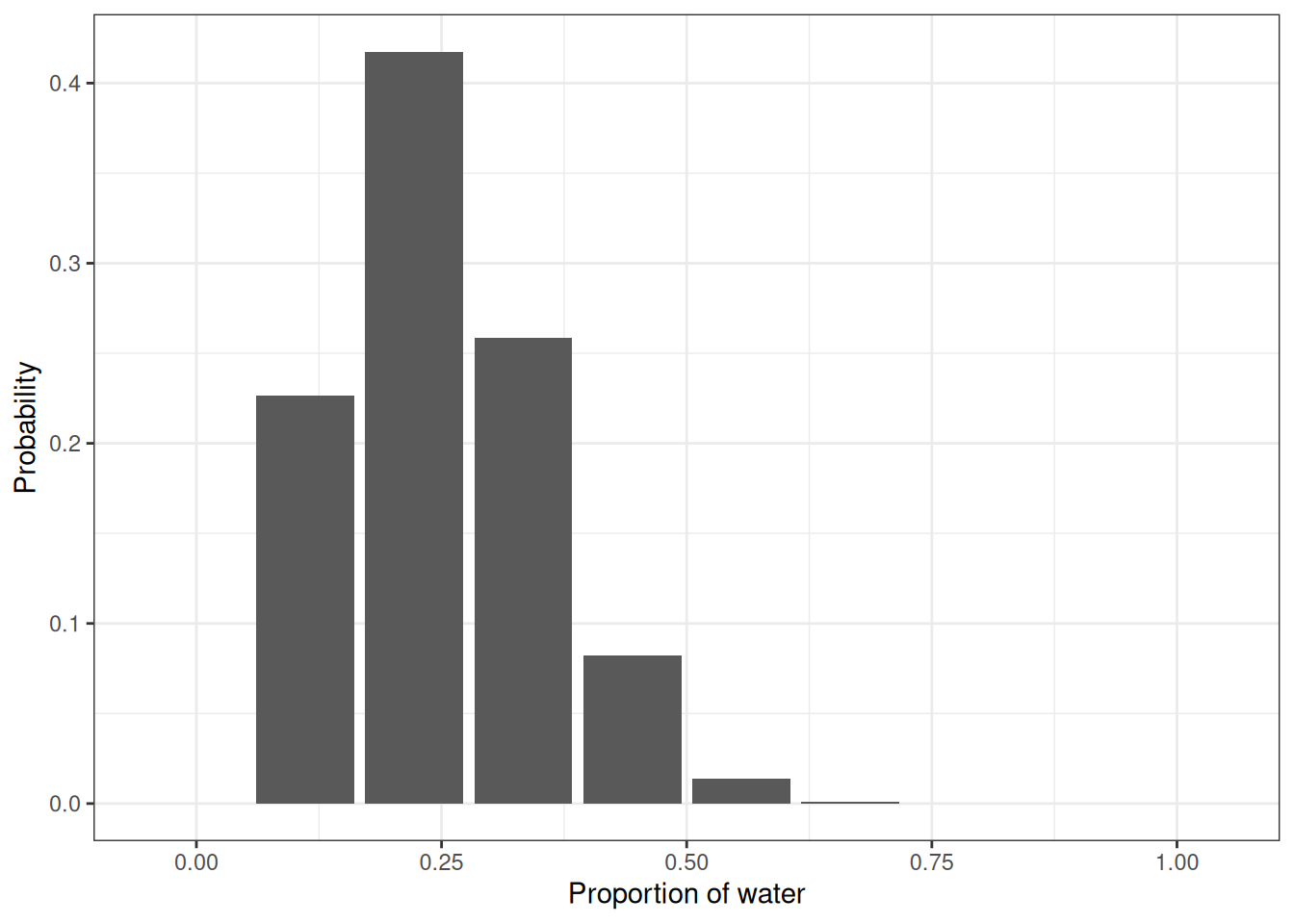
1. Suppose the globe tossing data (Lecture 2, Chapter 2) had turned out to be 3 water and 11 land. Construct the posterior distribution.

# Set number of water and land samples
n_water <- 3
n_land <- 11

# Set sequence of possible proportions
seq_prop <- seq(0, 1, length.out = 10)

# Count number of ways the sample could be produced for each possible proportion
n_ways <- globe_toss_n_ways(n_water, n_land, seq_prop)

# Compute the posterior distribution as the number of ways / sum of number of ways
posterior <- globe_toss_posterior(n_ways)

# Q1 data.frame
q1 <- data.frame(prob_prop = posterior,
                                 prop = seq_prop)

# Q1 plot
ggplot(q1) + 
    geom_col(aes(seq_prop, prob_prop)) + 
    labs(x = 'Proportion of water', y = 'Probability')

# Function: globe_toss_n_ways
globe_toss_n_ways

function (w, l, seq_prop) 
{
    ways_formula <- function(w, l, prop) {
        (prop^w) * (1 - prop)^l
    }
    vapply(seq_prop, function(p) {
        ways_formula(w, l, p)
    }, FUN.VALUE = 42)
}

# Function: globe_toss_posterior
globe_toss_posterior

function (n_ways) 
{
    n_ways/sum(n_ways)
}

Question 2

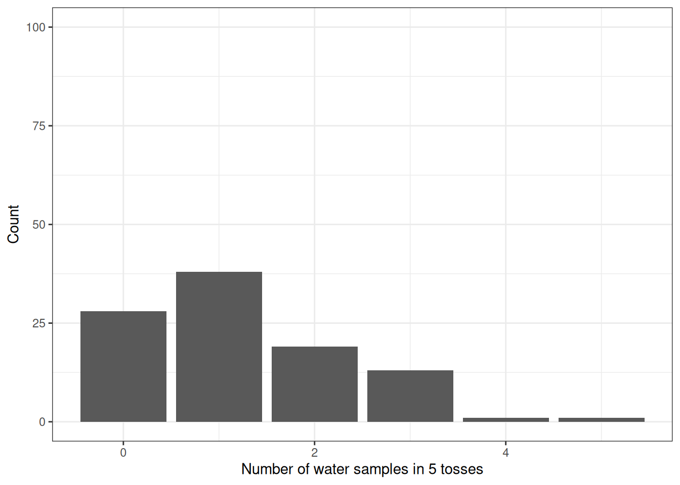
Using the posterior distribution from 1, compute the posterior predictive distribution for the next 5 tosses of the same globe. I recommend you use the sampling method.

# Take samples from the sequence of proportions using the 
#   probability defined in the posterior distribution
size <- 100
posterior_samples <- sample(
    q1$prop,
    size = size,
    prob = q1$prob_prop,
    replace = TRUE
)

# With the samples from the posterior distribution, 
#   simulate 5 tosses with each sampled probability probability
#   Binomial distributions are defined using 
#   a number of events and a probability of success
n_tosses <- 5
posterior_predict <- rbinom(size, size = n_tosses, p = posterior_samples)

# Plot number of W tosses
q2 <- data.frame(post_pred = posterior_predict)

# Plot
ggplot(q2) + 
    geom_bar(aes(x = post_pred)) +
    labs(x = 'Number of water samples in 5 tosses',
             y = 'Count') + 
    ylim(0, size)

Question 3 (optional)

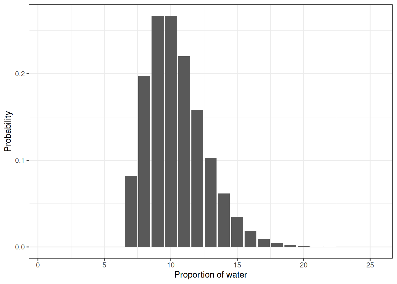
This problem is an optional challenge for people who are taking the course for a second or third time. uppose you observe W = 7 water points, but you forgot to write down how many times the globe was tossed, so you don’t know the number of land points L. Assume that p = 0.7 and compute the posterior distribution of the number of tosses N. Hint: Use the binomial distribution

n_water <- 7
n_land <- NA
p <- 0.7
n_tosses <- 5

n_samples <- seq(1, 25)

post <- vapply(n_samples, function(n) {
    dbinom(n_water, size = n, prob = p)
}, FUN.VALUE = 42)

q3 <- data.frame(n_prop = post, n = n_samples)

ggplot(q3) + 
    geom_col(aes(n_samples, n_prop)) + 
    labs(x = 'Proportion of water', y = 'Probability')