targets::tar_source('R')Homework 02
Setup
Question 1
From the Howell1 dataset, consider only the people younger than 13 years old. Estimate the causal association between age and weight. Assume that age influences weight through two paths. First, age influences height, and height influences weight. Second, age directly influences weight through age- related changes in muscle growth and body proportions.
Draw the DAG that represents these causal relationships. And then write a generative simulation that takes age as an input and simulates height and weight, obeying the relationships in the DAG.
coords <- data.frame(
    name = c('H', 'A', 'W'),
    x =    c(2,    1,   1),
    y =    c(1,    2,   0)
)

dagify(
    W ~ H + A,
    H ~ A,
  coords = coords
) |> ggdag(seed = 2) + theme_dag()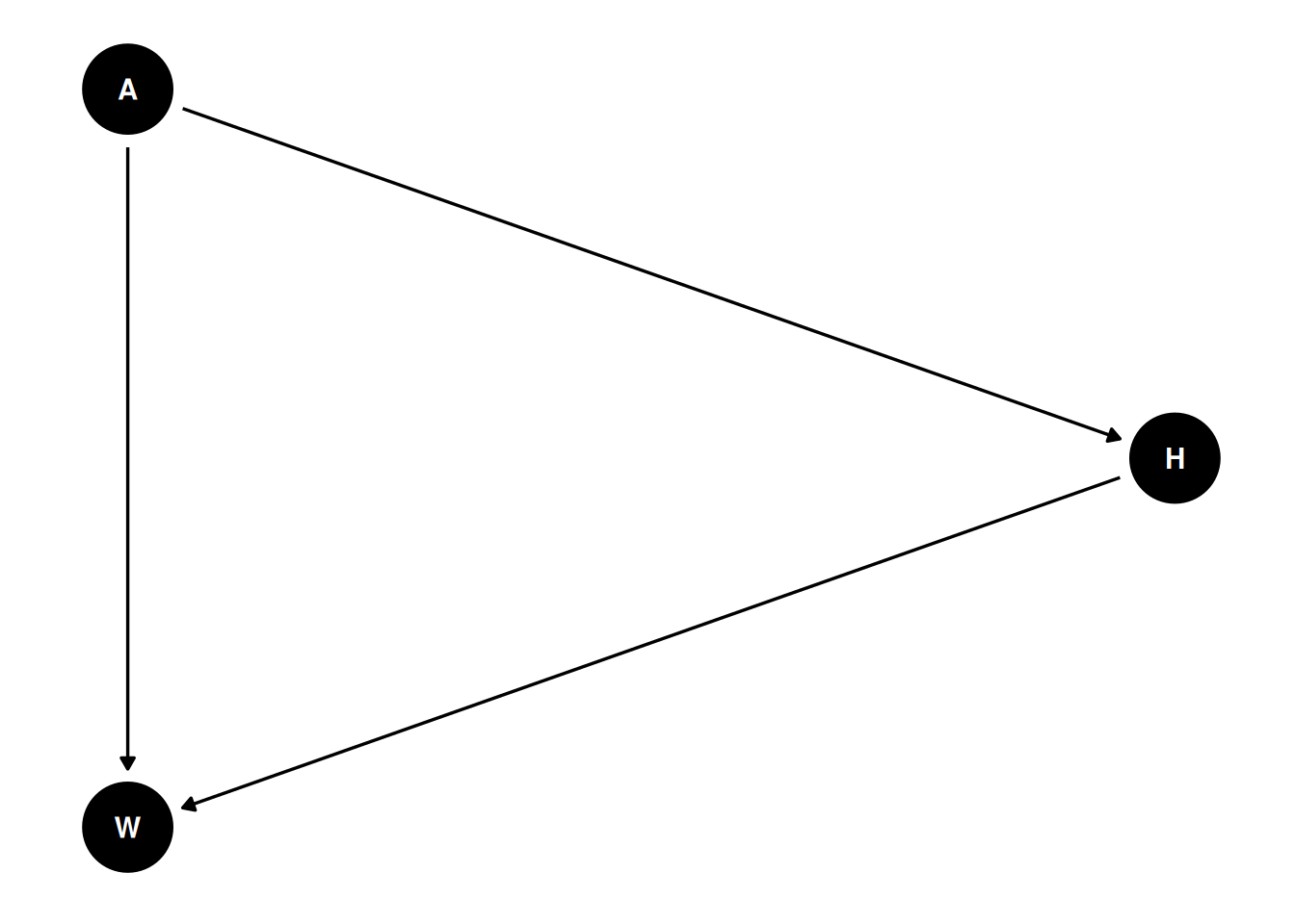
n <- 1e2
max_age <- 13

simulate_hw <- function(n, max_age) {
    age <- runif(n, 0, max_age)

    # General vague height at 13 years old (cm) = 130
    beta_age_on_height <- 10
    height <- rnorm(n = n, mean = age * beta_age_on_height, 2)

    # General vague weight at 13 years old (kg) = 45
    # Betas chosen to hit 45 kg approximately at 13 years old
    beta_height_on_weight <- 0.2
    beta_age_on_weight <- 1.5
    weight <- (age * beta_age_on_weight) +
        (beta_height_on_weight * height)

    data.table(age, height, weight)
}
ggplot(simulate_hw(n, max_age)) +
    geom_point(aes(age, weight))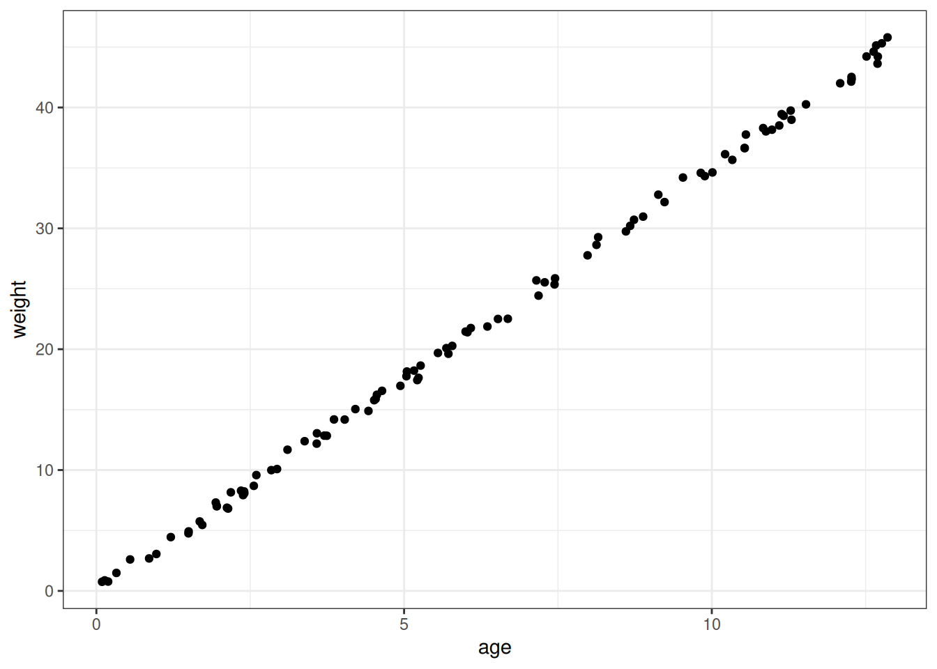
Question 2
Estimate the total causal effect of each year of growth on weight.
The total causal effect of age on weight is estimated by excluding the height variable to include both paths in the DAG from age to weight directly and indirectly through height (Lecture 4: slide 28).
Prior predictive simulation
# Function for preparing Howell data
data_Howell
function() {
if (!'rethinking' %in% .packages()) {
stop('please load the rethinking package')
}
if (!'data.table' %in% .packages()) {
stop('please load the data.table package')
}
data(Howell1)
DT <- data.table::data.table(Howell1)
DT[, sex := .GRP, by = male]
DT[, scale_height := scale(height)]
DT[, scale_weight := scale(weight)]
DT[, scale_height_div_mean := height / mean(height)]
DT[, scale_weight_div_mean := weight / mean(weight)]
return(DT)
}# Load data
DT <- tar_read(Howell_lte_13)
# Print priors used
tar_read(h02_q02_brms_prior) prior class coef group resp dpar nlpar lb ub source
normal(22.5, 0.5) Intercept <NA> <NA> user
normal(3, 0.5) b <NA> <NA> user
exponential(1) sigma <NA> <NA> user# Load model
tar_load(h02_q02_brms_sample_prior)
h02_q02_brms_sample_prior Family: gaussian
Links: mu = identity; sigma = identity
Formula: weight ~ age
Data: h02_q02_brms_data (Number of observations: 157)
Draws: 4 chains, each with iter = 2000; warmup = 1000; thin = 1;
total post-warmup draws = 4000
Regression Coefficients:
Estimate Est.Error l-95% CI u-95% CI Rhat Bulk_ESS Tail_ESS
Intercept 4.74 3.10 -1.40 10.63 1.00 2994 2474
age 2.99 0.51 2.02 3.99 1.00 3047 2383
Further Distributional Parameters:
Estimate Est.Error l-95% CI u-95% CI Rhat Bulk_ESS Tail_ESS
sigma 0.99 0.98 0.02 3.59 1.00 2148 1209
Draws were sampled using sample(hmc). For each parameter, Bulk_ESS
and Tail_ESS are effective sample size measures, and Rhat is the potential
scale reduction factor on split chains (at convergence, Rhat = 1).# Read N draws from the priors and append expected predictions
n_draws <- 50
q02_draws <- h02_q02_brms_sample_prior |>
add_epred_draws(newdata = unique(DT[, .(age)]),
ndraws = n_draws)
# Plot prior expectations for relationship between age and weight
ggplot(q02_draws) +
geom_line(aes(age, .epred, group = .draw), alpha = 0.5) +
labs(x = 'Age', y = 'Weight')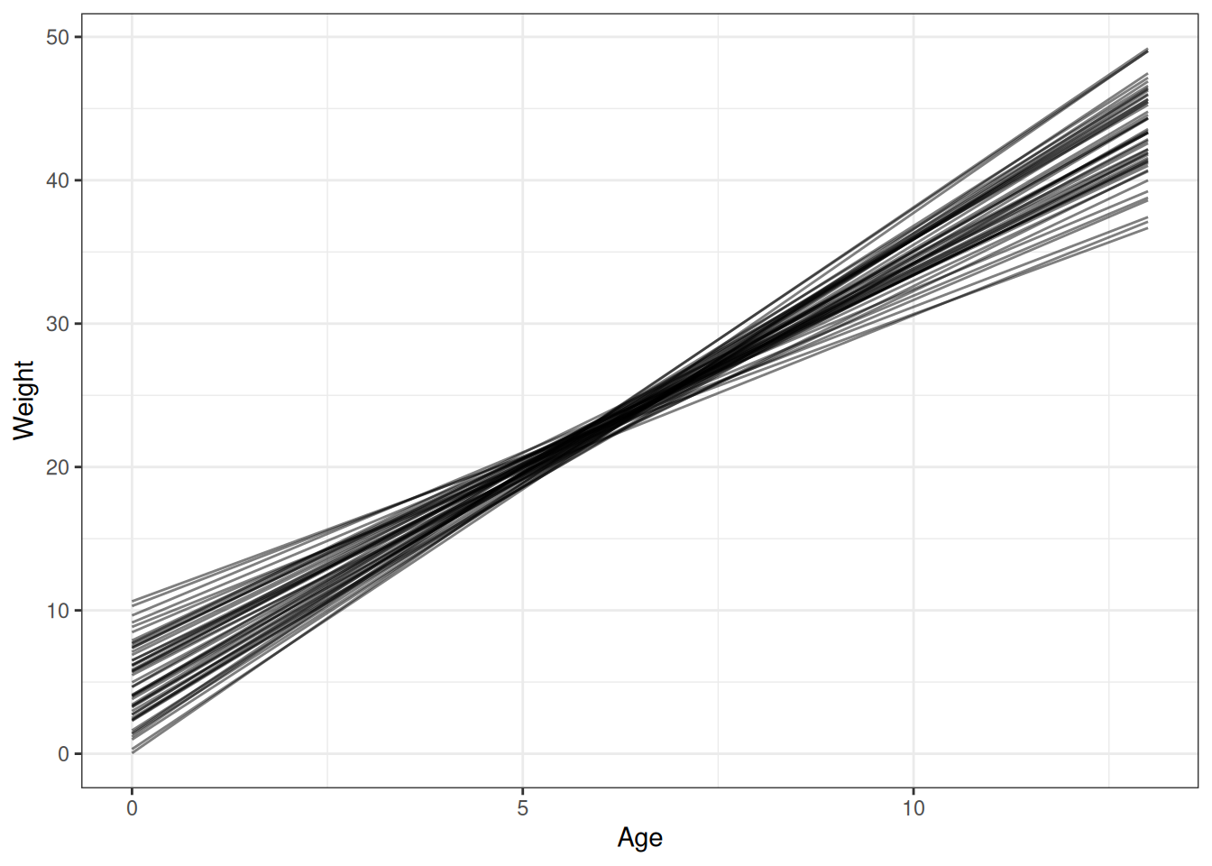
Analyse the data
# Load model
tar_load(h02_q02_brms_sample)
h02_q02_brms_sample
Family: gaussian
Links: mu = identity; sigma = identity
Formula: weight ~ age
Data: h02_q02_brms_data (Number of observations: 157)
Draws: 4 chains, each with iter = 2000; warmup = 1000; thin = 1;
total post-warmup draws = 4000
Regression Coefficients:
Estimate Est.Error l-95% CI u-95% CI Rhat Bulk_ESS Tail_ESS
Intercept 8.55 0.41 7.77 9.37 1.00 3004 2831
age 1.35 0.05 1.24 1.46 1.00 3259 2290
Further Distributional Parameters:
Estimate Est.Error l-95% CI u-95% CI Rhat Bulk_ESS Tail_ESS
sigma 2.83 0.20 2.47 3.27 1.00 2708 2595
Draws were sampled using sample(hmc). For each parameter, Bulk_ESS
and Tail_ESS are effective sample size measures, and Rhat is the potential
scale reduction factor on split chains (at convergence, Rhat = 1).# Tidy draws
q02_draws <- h02_q02_brms_sample |>
tidy_draws()
q02_newdata <- data_grid(DT, age = seq_range(age, 20))
q02_epred <- h02_q02_brms_sample |>
epred_draws(q02_newdata)
# Total causal effect of each year of growth on weight
g1 <- ggplot(q02_draws) +
stat_halfeye(aes(b_age)) +
labs(x = 'Increase in weight per year of growth', y = '')
g2 <- ggplot(q02_epred) +
stat_ribbon(aes(age, .epred), alpha = 0.5) +
scale_fill_grey(start = 0.8, end = 0.2) +
labs(x = 'Age', y = 'Weight')
g1 / g2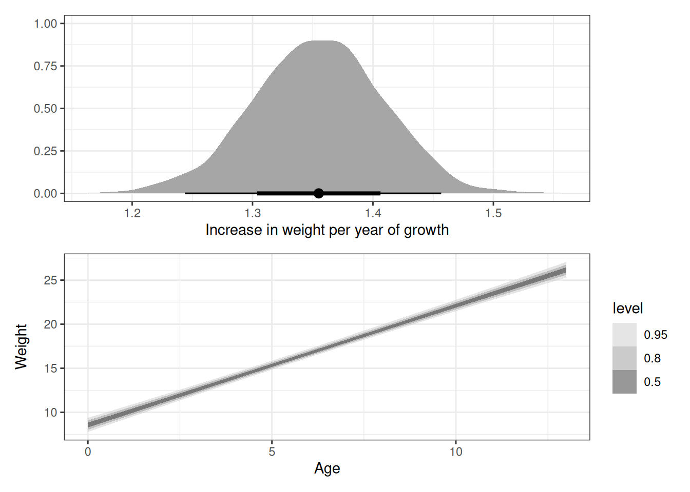
Question 3
The data in data(Oxboys) (rethinking package) are growth records for 26 boys measured over 9 periods. I want you to model their growth. Specifically, model the increments in growth from one period (Occasion in the data table) to the next. Each increment is simply the difference between height in one occasion and height in the previous occasion. Since none of these boys shrunk during the study, all of the growth increments are greater than zero. Estimate the posterior distribution of these increments. Constrain the distribution so it is always positive—it should not be possible for the model to think that boys can shrink from year to year. Finally compute the posterior distribution of the total growth over all 9 occasions.
Prior predictive simulation
# Function for preparing Oxboys data
data_Oxboys
function() {
if (!'rethinking' %in% .packages()) {
stop('please load the rethinking package')
}
if (!'data.table' %in% .packages()) {
stop('please load the data.table package')
}
data("Oxboys")
DT <- data.table::data.table(Oxboys)
DT[, diff_height := height - shift(height), by = Subject]
DT[, occasion_factor := factor(Occasion)]
return(DT)
}# Load data
DT <- tar_read(prep_Oxboys)
# Print priors used
tar_read(h02_q03_brms_prior) prior class coef group resp dpar nlpar lb ub source
normal(5, 2) Intercept <NA> <NA> user
normal(3, 1) b <NA> <NA> user
exponential(1) sigma <NA> <NA> user# Load model
tar_load(h02_q03_brms_sample_prior)
h02_q03_brms_sample_prior Family: gaussian
Links: mu = identity; sigma = identity
Formula: diff_height | trunc(lb = 0) ~ occasion_factor
Data: h02_q03_brms_data (Number of observations: 208)
Draws: 4 chains, each with iter = 2000; warmup = 1000; thin = 1;
total post-warmup draws = 4000
Regression Coefficients:
Estimate Est.Error l-95% CI u-95% CI Rhat Bulk_ESS Tail_ESS
Intercept 2.38 2.01 -1.56 6.43 1.00 7337 2974
occasion_factor3 3.01 1.02 1.02 4.99 1.00 6519 2990
occasion_factor4 3.01 1.00 1.02 4.94 1.00 8041 2922
occasion_factor5 3.00 1.01 1.06 5.00 1.00 7578 2782
occasion_factor6 3.01 0.97 1.17 4.93 1.00 6750 3239
occasion_factor7 3.00 1.01 1.03 4.94 1.00 7103 3230
occasion_factor8 3.00 0.97 1.07 4.92 1.00 7255 3110
occasion_factor9 2.98 1.01 1.01 4.99 1.00 6316 2813
Further Distributional Parameters:
Estimate Est.Error l-95% CI u-95% CI Rhat Bulk_ESS Tail_ESS
sigma 1.00 1.00 0.02 3.62 1.00 4453 1966
Draws were sampled using sample(hmc). For each parameter, Bulk_ESS
and Tail_ESS are effective sample size measures, and Rhat is the potential
scale reduction factor on split chains (at convergence, Rhat = 1).# Read N draws from the priors and append expected predictions
n_draws <- 100
q02_newdata <- data_grid(DT, age = seq_range(age, 20))
q03_newdata <- na.omit(DT)[, .(occasion_factor = droplevels(unique(occasion_factor)))]
q03_epred_prior <- h02_q03_brms_sample_prior |>
add_epred_draws(newdata = q03_newdata, ndraws = n_draws)
# Plot prior expectations for relationship between occasion and height
ggplot(q03_epred_prior) +
stat_halfeye(aes(occasion_factor, .epred), alpha = 0.5) +
labs(x = 'Occasion', y = 'Difference in height')Warning: Computation failed in `stat_slabinterval()`.
Caused by error in `seq.default()`:
! 'to' must be a finite number
Analyse the data
# Load model
tar_load(h02_q03_brms_sample)
h02_q03_brms_sample
Family: gaussian
Links: mu = identity; sigma = identity
Formula: diff_height | trunc(lb = 0) ~ occasion_factor
Data: h02_q03_brms_data (Number of observations: 208)
Draws: 4 chains, each with iter = 2000; warmup = 1000; thin = 1;
total post-warmup draws = 4000
Regression Coefficients:
Estimate Est.Error l-95% CI u-95% CI Rhat Bulk_ESS Tail_ESS
Intercept 0.82 0.27 0.21 1.29 1.01 677 732
occasion_factor3 0.56 0.31 -0.01 1.21 1.01 1042 1299
occasion_factor4 1.03 0.32 0.47 1.70 1.01 940 1098
occasion_factor5 0.09 0.32 -0.50 0.75 1.00 1184 1608
occasion_factor6 0.42 0.32 -0.18 1.06 1.01 1119 1379
occasion_factor7 1.46 0.32 0.90 2.15 1.01 918 1014
occasion_factor8 1.21 0.32 0.62 1.90 1.01 935 1074
occasion_factor9 0.71 0.31 0.13 1.37 1.01 940 1060
Further Distributional Parameters:
Estimate Est.Error l-95% CI u-95% CI Rhat Bulk_ESS Tail_ESS
sigma 0.93 0.08 0.79 1.10 1.00 1180 1385
Draws were sampled using sample(hmc). For each parameter, Bulk_ESS
and Tail_ESS are effective sample size measures, and Rhat is the potential
scale reduction factor on split chains (at convergence, Rhat = 1).# Expectation draws
q03_epred <- h02_q03_brms_sample |>
add_epred_draws(newdata = q03_newdata, ndraws = n_draws)
# Plot posterior expectations for relationship between occasion and height
ggplot(q03_epred) +
stat_halfeye(aes(occasion_factor, .epred), alpha = 0.5) +
labs(x = 'Occasion', y = 'Difference in height')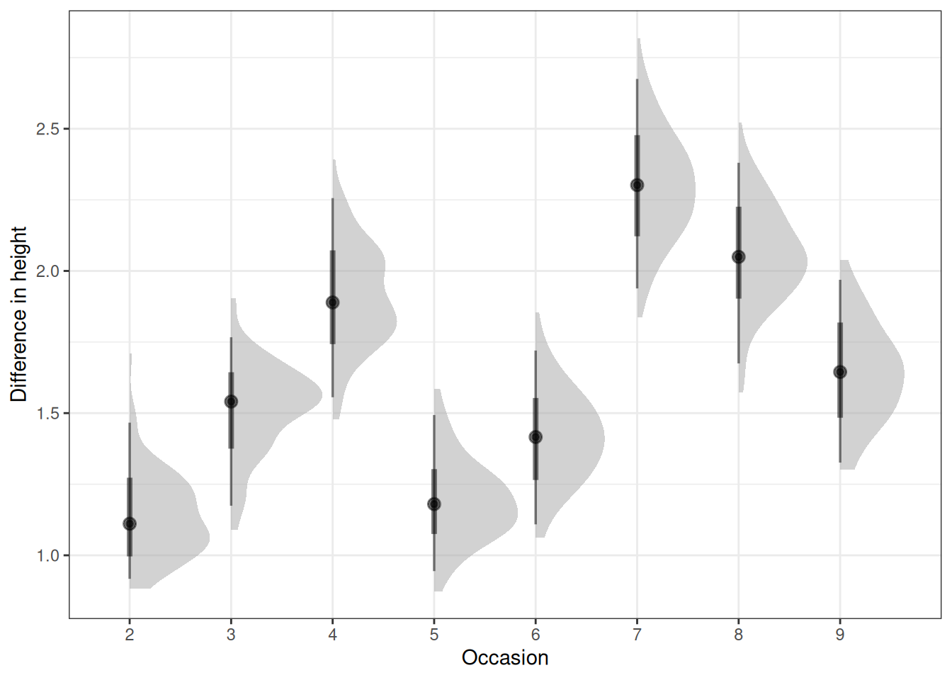
# Tidy draws
q03_draws  <- h02_q03_brms_sample |>
    tidy_draws() |>
    data.table()

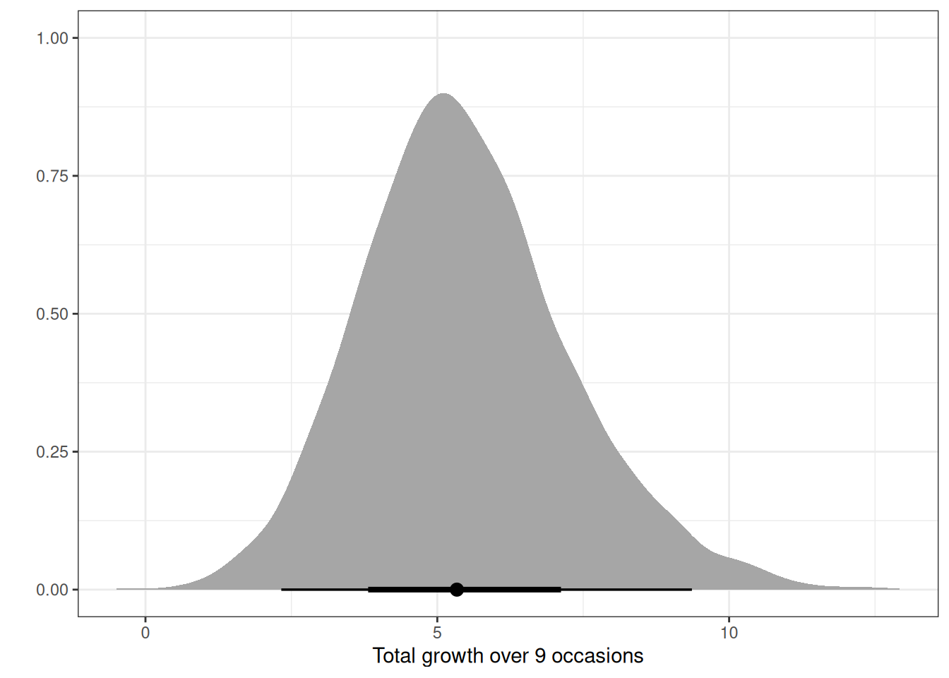
# Calculate total growth
q03_draws[, total_growth := rowSums(.SD), .SDcols = patterns('b_occasion')]

ggplot(q03_draws) +
    stat_halfeye(aes(total_growth)) +
    labs(x = 'Total growth over 9 occasions', y = '')