targets::tar_source('R')Homework 04
Setup
Question 1
Revisit the marriage, age, and happiness collider bias example from Chapter 6. Run models m6.9 and m6.10 again (pages 178–179). Compare these two models using both PSIS and WAIC. Which model is expected to make better predictions, according to these criteria, and which model yields the correct causal inference?
tar_load(h04_q01_m6_9_brms_sample)
tar_load(h04_q01_m6_10_brms_sample)

m6_9_loo <- add_criterion(h04_q01_m6_9_brms_sample, 'loo')
m6_10_loo <- add_criterion(h04_q01_m6_10_brms_sample, 'loo')

loo_compare(m6_9_loo, m6_10_loo)
elpd_diff se_diff
m6_9_loo 0.0 0.0
m6_10_loo -194.1 17.6 The criterion of model fit selected is the Bayesian LOO estimate of the expected log pointwise predictive density (ELPD). The model with the highest LOO ELPD is model 6.9 which includes a known collider: marriage status. Model 6.9 is expected to make better predictions but not expected to yield the correct causal inference. Model 6.10 without marriage status has a lower LOO ELPD, “a coarse measure of uncertainty about the predictive performance of unknown future data” ({loo} glossary), but is expected to yield the correct causal inference.
Question 2
Reconsider the urban fox analysis from last week’s homework. On the basis of PSIS and WAIC scores, which combination of variables best predicts body weight (W, weight)? What causal interpretation can you assign each coefficient (parameter) from the best scoring model?
All combinations of the three variables, area, average food, and group size:
- Area
- Average food (H03 Q02)
- Group size
- Area, average food
- Area, group size
- Average food, group size (H03 Q03)
- Area, average food, group size
q02_m1 <- tar_read(h04_q02_m_1_brms_sample) |> add_criterion('loo')
q02_m2 <- tar_read(h03_q02_brms_sample) |> add_criterion('loo')
q02_m3 <- tar_read(h04_q02_m_3_brms_sample) |> add_criterion('loo')
q02_m4 <- tar_read(h04_q02_m_4_brms_sample) |> add_criterion('loo')
q02_m5 <- tar_read(h04_q02_m_5_brms_sample) |> add_criterion('loo')
q02_m6 <- tar_read(h03_q03_brms_sample) |> add_criterion('loo')
q02_m7 <- tar_read(h04_q02_m_7_brms_sample) |> add_criterion('loo')

loo_compare(
    q02_m1,
    q02_m2,
    q02_m3,
    q02_m4,
    q02_m5,
    q02_m6,
    q02_m7
)
elpd_diff se_diff
q02_m7 0.0 0.0
q02_m5 -0.4 1.6
q02_m6 -0.5 1.7
q02_m3 -3.9 3.0
q02_m2 -5.2 3.6
q02_m1 -5.4 3.7
q02_m4 -5.8 3.5 The best combination of variables on the basis of prediction is: all three.
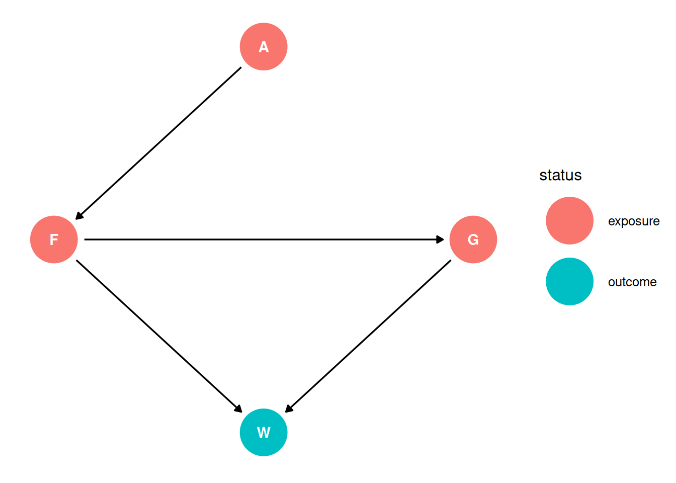
dag <- dagify(
    G ~ F,
    F ~ A,
    W ~ F + G,
  coords = coords,
    exposure = c('F', 'G', 'A'),
    outcome = 'W'
)
ggdag_status(dag, seed = 2, layout = 'auto') + theme_dag()
Taking each variable in turn, we can consider the causal interpretations of each:
| Variable | Direct effect | Total effect | Interpretation variable in the context of W ~ A + F + G |
|---|---|---|---|
| Area (A) | When estimating the direct effect of A on W, there is a biasing path through F. If F is included, the direct effect of A on W can be estimated. | No other variables should be included when estimating the total effect of A on W. | Coefficient indicates the direct effect of A on W but F is a mediator or pipe along the path which should, if the DAG is correctly representing the system, result in no association between A and W. |
| Average food (F) | When estimating the direct effect of F on W, there is a biasing path through G. If G is included, the direct effect of F on W can be estimated. | G should not be included when estimating the total effect of F on W. | Coefficient indicates the direct effect of F on W. |
| Group size (G) | When estimating the direct effect of G on W, there is a biasing path through F. If F is included, the direct effect of G on W can be estimated. | G must be included to estimate the total effect of G on W. | Coefficient indicates the direct effect of G on W. |
Question 3
The data in data(Dinosaurs) are body mass estimates at different estimated ages for six different dinosaur species. See ?Dinosaurs for more details. Choose one or more of these species (at least one, but as many as you like) and model its growth. To be precise: Make a predictive model of body mass using age as a predictor. Consider two or more model types for the function relating age to body mass and score each using PSIS and WAIC. Which model do you think is best, on predictive grounds? On scientific grounds? If your answers to these questions differ, why? This is a challenging exercise, because the data are so scarce. But it is also a realistic example, because people publish Nature papers with even less data. So do your best, and I look forward to seeing your growth curves.
m_lin <- tar_read(h04_q03_m_lin_Massos_brms_sample) |> add_criterion('loo')Warning: Found 2 observations with a pareto_k > 0.7 in model
'tar_read(h04_q03_m_lin_Massos_brms_sample)'. We recommend to set 'moment_match
= TRUE' in order to perform moment matching for problematic observations.m_exp <- tar_read(h04_q03_m_exp_Massos_brms_sample) |> add_criterion('loo')Warning: Found 2 observations with a pareto_k > 0.7 in model
'tar_read(h04_q03_m_exp_Massos_brms_sample)'. We recommend to set 'moment_match
= TRUE' in order to perform moment matching for problematic observations.m_wei <- tar_read(h04_q03_m_wei_Massos_brms_sample) |> add_criterion('loo')Warning: Found 2 observations with a pareto_k > 0.7 in model
'tar_read(h04_q03_m_wei_Massos_brms_sample)'. We recommend to set 'moment_match
= TRUE' in order to perform moment matching for problematic observations.loo_compare(
m_lin,
m_exp,
m_wei
) elpd_diff se_diff
m_exp 0.0 0.0
m_wei -0.9 9.5
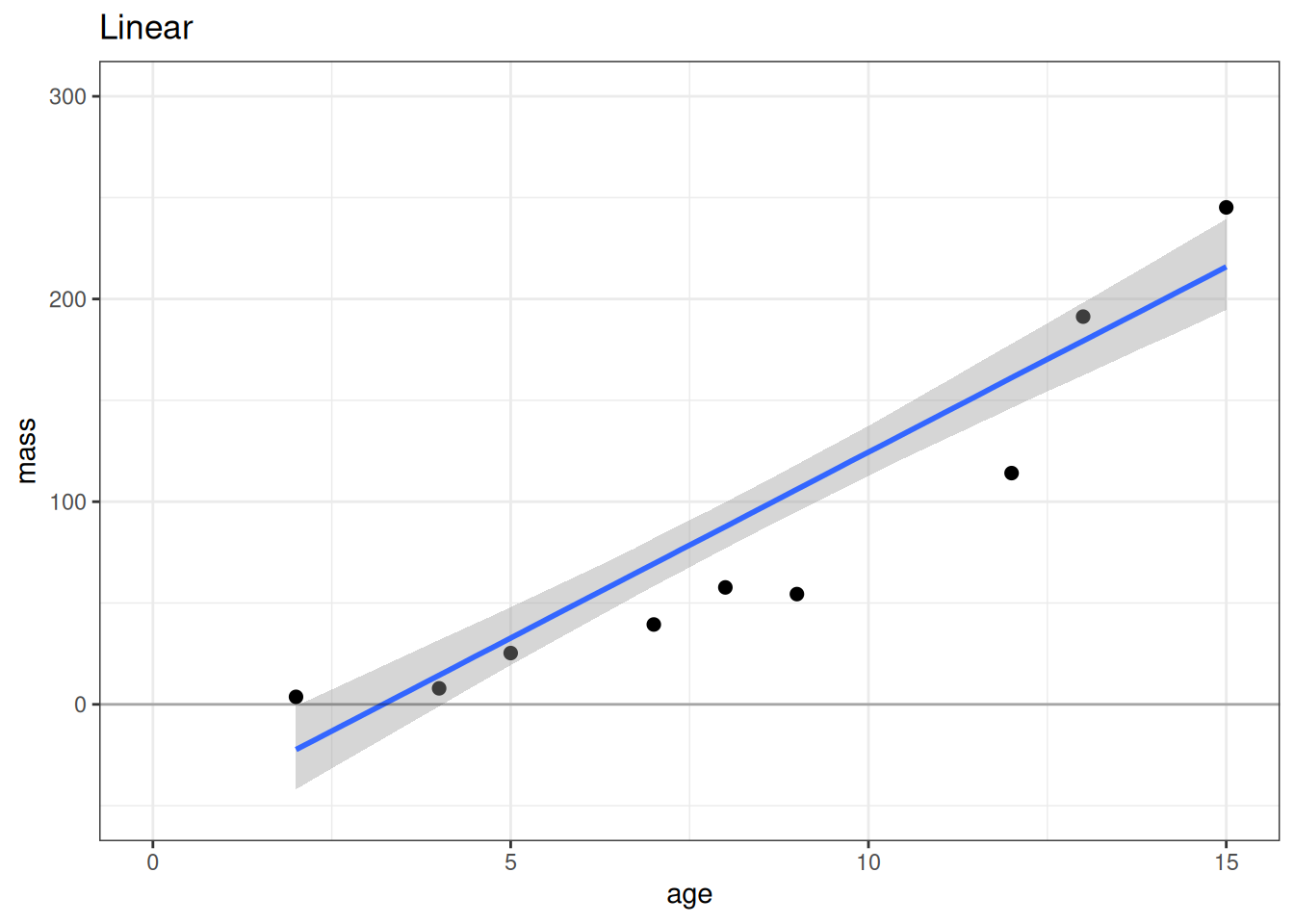
m_lin -8.0 10.1 theme_set(theme_bw())
# Linear
plot(conditional_effects(m_lin), points = TRUE, plot = FALSE)[[1]] +
lims(x = c(0, 15), y = c(-50, 300)) +
geom_hline(yintercept = 0, alpha = 0.3) +
labs(title = 'Linear')
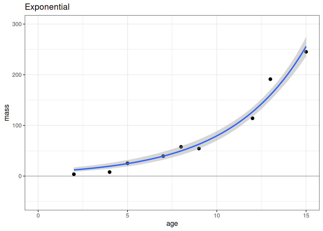
# Exponential
plot(conditional_effects(m_exp), points = TRUE, plot = FALSE)[[1]] +
    lims(x = c(0, 15), y = c(-50, 300)) +
    geom_hline(yintercept = 0, alpha = 0.3) +
    labs(title = 'Exponential')
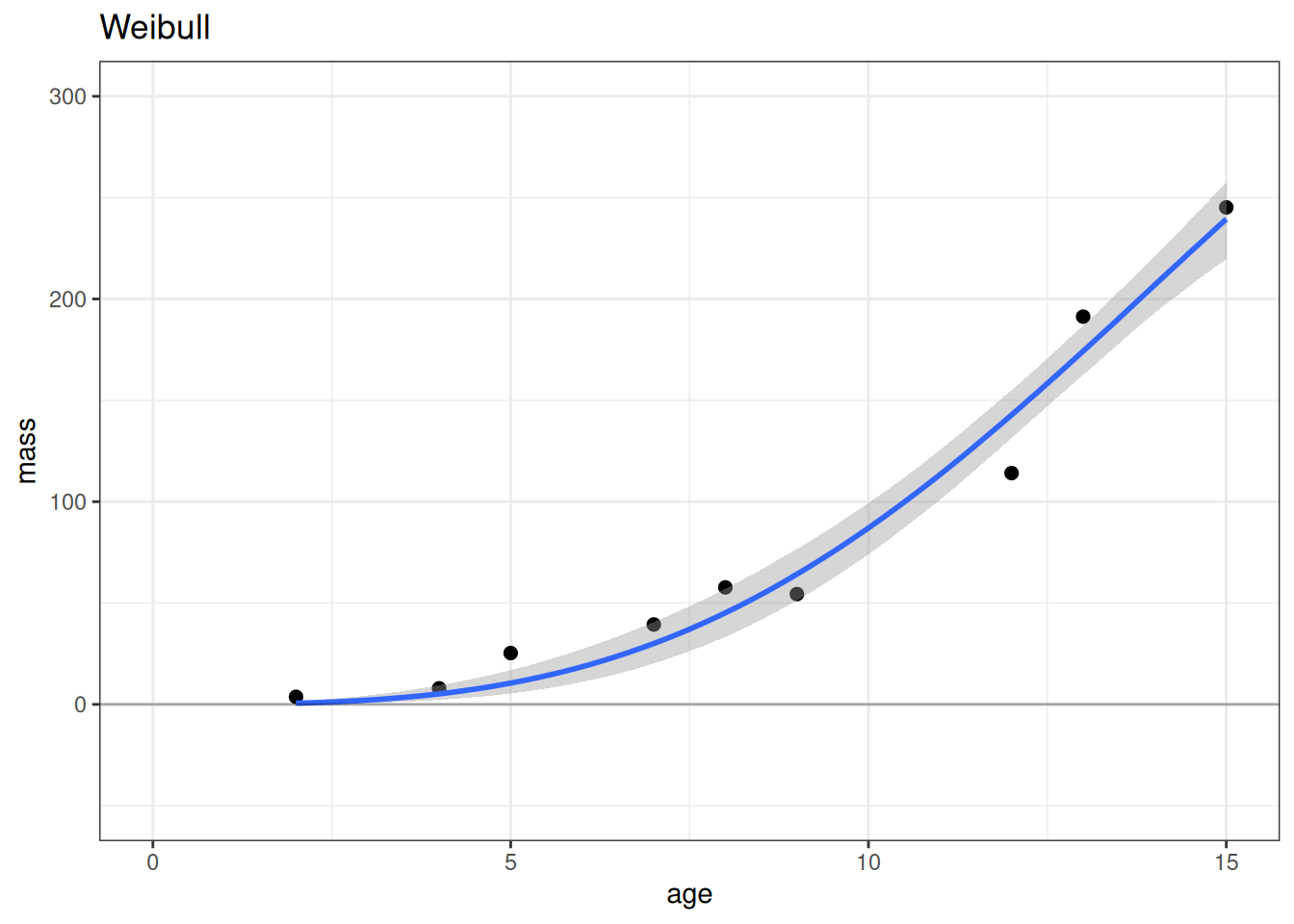
# Weibull
plot(conditional_effects(m_wei), points = TRUE, plot = FALSE)[[1]] +
    lims(x = c(0, 15), y = c(-50, 300)) +
    geom_hline(yintercept = 0, alpha = 0.3) +
    labs(title = 'Weibull')
According to the LOO ELPD, the most predictive model is the exponential model followed closely by the Weibull model. The linear model has worse model fit criterion (LOO ELPD) making it a worse model for prediction. On scientific grounds, we would also not expect a linear model to best describe the relationship between age and mass. Both the Weibull and exponential models have better expectations nearing age 0, while the linear model expects that mass should be negative at young ages.
Resources:
- https://paul-buerkner.github.io/brms/articles/brms_nonlinear.html
- https://journal.r-project.org/archive/2018/RJ-2018-017/RJ-2018-017.pdf
- https://www.magesblog.com/post/2015-11-03-loss-developments-via-growth-curves-and/
- https://en.wikipedia.org/wiki/Exponential_function