dag <- dagify(
S ~ Q + J,
Q ~ X,
J ~ Z,
coords = coords,
exposure = 'Q',
outcome = 'S',
latent = c('Q', 'J')
)
ggdag(dag, seed = 2, layout = 'auto') + theme_dag()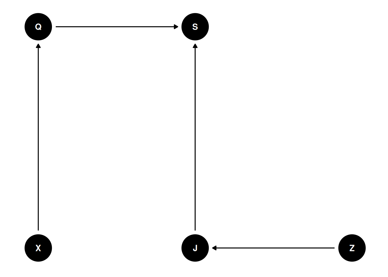
Use in Bayesian statistics: to draw samples from a distribution
Sample each parameter value in proportion to its probability
There can be any number of dimensions (parameters)
At every step, the comparison is between the current combination of parameter values, and the candidate combination of parameter values. In this way, we don’t need to evaluate the entire grid
Simple version of Markov chain Monte Carlo (MCMC)
Modern, open source, high-performance statistical computation tool.
data {
    // the observed variables
    vector[50] D;
    vector[50] A;
    vector[50] M;
}
parameters {
    // the unobserved variables
    real a;
    real bM;
    real bA;
    real<lower=0> sigma;
}
model {
    // compute the log posterior probability
    vector[50] mu;
    sigma ~ exponential( 1 );
    bA ~ normal( 0 , 0.5 );
    bM ~ normal( 0 , 0.5 );
    a ~ normal( 0 , 0.2 );
    for ( i in 1:50 ) {
        mu[i] = a + bM * M[i] + bA * A[i];
    }
    D ~ normal( mu , sigma );
}“When you have computation problems, often there’s a problem with your model” - Andrew Gelman
By problems with the models, he is referring to the probability assumptions, the priors, the statistical assumptions
This is an example of modeling latent variables and item response models.
dag <- dagify(
    S ~ Q + J,
    Q ~ X,
    J ~ Z,
  coords = coords,
    exposure = 'Q',
    outcome = 'S',
  latent = c('Q', 'J')
)
ggdag(dag, seed = 2, layout = 'auto') + theme_dag()
Wine quality (Q) is a latent variable meaning it is unobserved. There is no way to directly measure the quality of a wine because that is determined by preferences, etc.
We can observe the score (S) given by judges, who each have their own unobservable characteristics such as dispositions, opinions, biases, etc. Wine origin may affect the wine quality and the score (which may occur if judges’ origin biases them to wine origin).
If the blinding is not 100% accurate, if judges can guess the origin of the wine, they may be biased.
What is the association between wine quality and wine origin, stratified by judge to improve precision of influence of wine origin?
In the lectures, Richard builds up the model in components, slowly adding complexity.
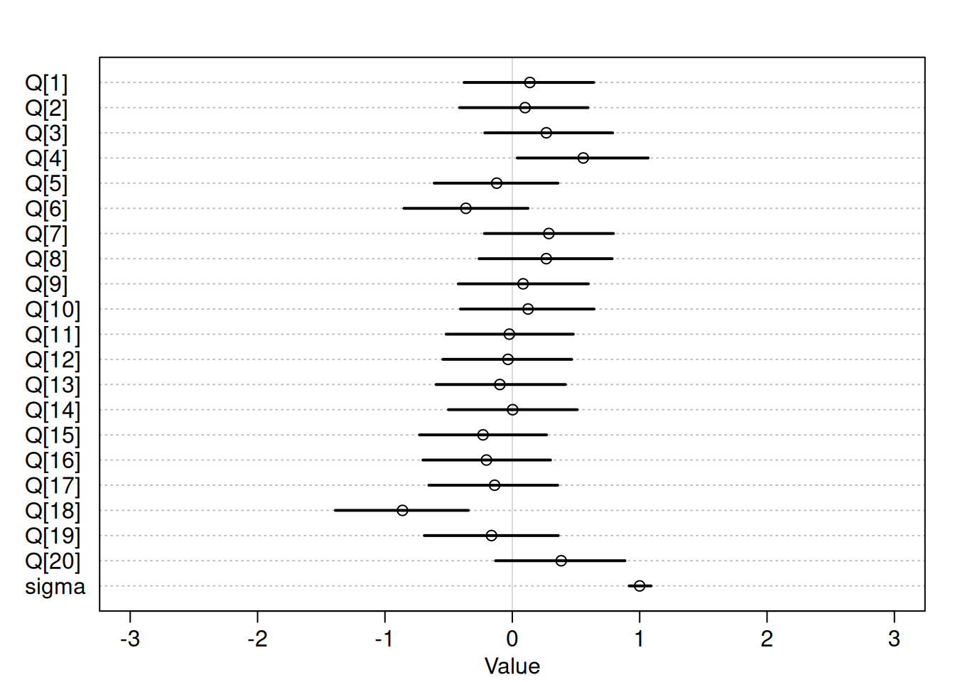
First, model the association of wine score with wine quality.
Wine quality is an unobserved parameter in the model. Since score is standardized, the average wine score will have an average quality.
\[S_{i} \sim Normal(\mu_{i}, \sigma)\] \[\mu_{i} = Q_{W[i]}\] \[Q_{j} \sim Normal(0, 1)\] \[\sigma \sim Exponential(1)\]
data(Wines2012)
d <- Wines2012
dat <- list(
    S = standardize(d$score),
    J = as.numeric(d$judge),
    W = as.numeric(d$wine),
    X = ifelse(d$wine.amer == 1, 1, 2),
    Z = ifelse(d$judge.amer == 1, 1, 2)
)
mQ <- ulam(
    alist(S ~ dnorm(mu, sigma),
                mu <- Q[W],
                Q[W] ~ dnorm(0, 1),
                sigma ~ dexp(1)),
    data = dat,
    chains = 4,
    cores = 4
)Note: there is variability in the estimate unobserved parameter Q across wines.
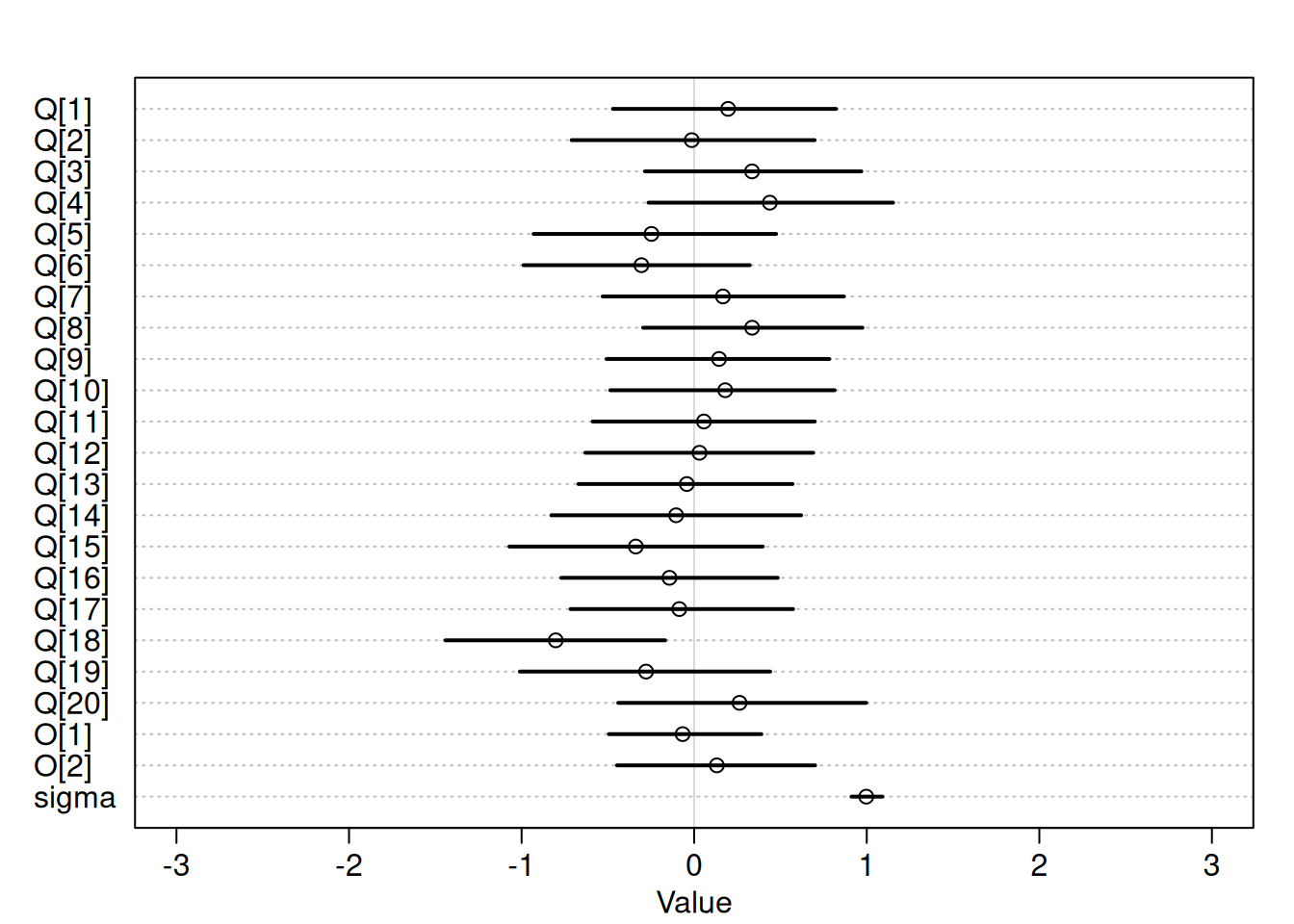
Next, add the wine origin variable and stratify by it.
\[S_{i} \sim Normal(\mu_{i}, \sigma)\] \[\mu_{i} = Q_{W[i]} + O_{X[i]}\] \[Q_{j} \sim Normal(0, 1)\] \[O_{j} \sim Normal(0, 1)\]
\[\sigma \sim Exponential(1)\]
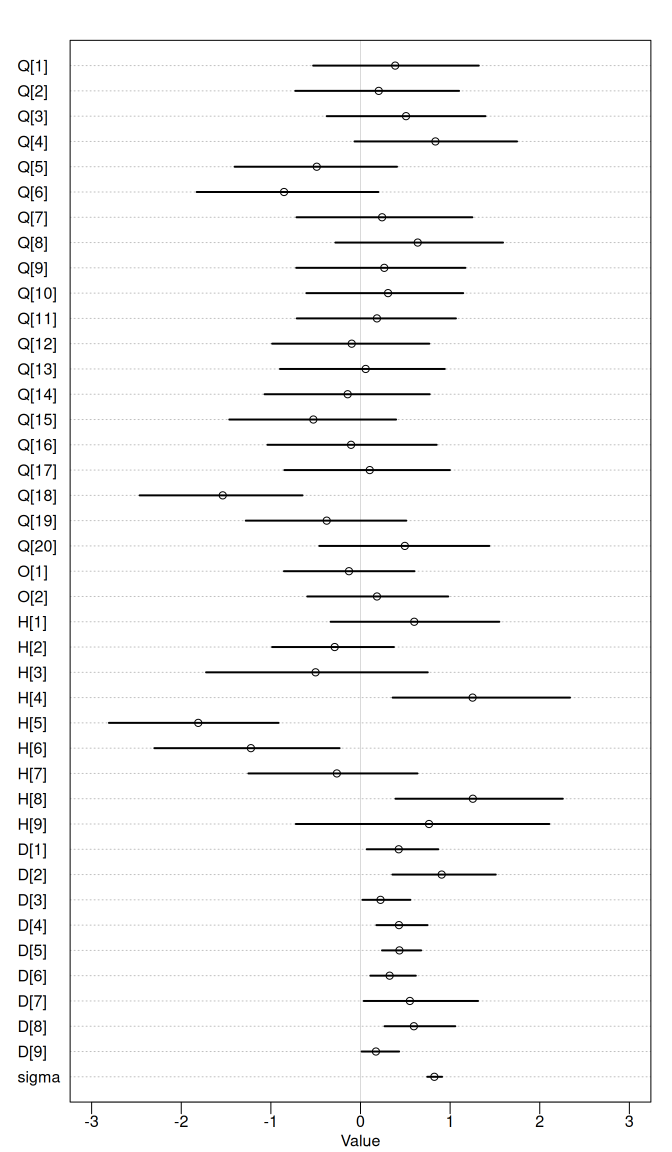
Lastly, introduce judge effects.
Judges’ biases are a competing cause and we use two additional latent variables (H and D) to measure them. \(\mu_{i}\) is the expected score of a wine and it is calculated by multiplying the judge discrimination (D) by wine quality added to origin (O) subtracted by judge harshness (H). Harshness represents how good a wine has to be to give it an average score. Discriminatory judges give very disperse scores to different wines, whereas non-discriminatory judges give similar scores to all wines. This formulation comes from common judge or item response models.
\[S_{i} \sim Normal(\mu_{i}, \sigma)\] \[\mu_{i} = (Q_{W[i]} + O_{X[i]} - H_{J[i]})D_{J[i]}\] \[Q_{j} \sim Normal(0, 1)\] \[O_{j} \sim Normal(0, 1)\] \[H_{j} \sim Normal(0, 1)\] \[D_{j} \sim Normal(0, 1)\] \[\sigma \sim Exponential(1)\]
We see a lot of variation between judges. Judge 4 has a high harshness value compared to judges 5 and 6. Including judge specific latent effects helps us provide better estimates by dealing with these known contributing causes of wine score.