targets::tar_source('R')Homework 05
Setup
Question 1
The data in data(NWOGrants) are outcomes for scientific funding applications for the Netherlands Organization for Scientific Research (NWO) from 2010–2012 (see van der Lee and Ellemers doi:10.1073/pnas.1510159112). These data have a structure similar to the UCBAdmit data discussed in Chapter 11 and in lecture. There are applications and each has an associated gender (of the lead researcher). But instead of departments, there are disciplines. Draw a DAG for this sample. Then use the backdoor criterion and a binomial GLM to estimate the TOTAL causal effect of gender on grant awards.
Estimand
What is the total causal effect of gender on grant awards?
Scientific model
dag <- dagify(
    D ~ G,
    A ~ G + D,
  coords = coords,
    exposure = 'G',
    outcome = 'A'
)
ggdag_status(dag, seed = 2, layout = 'auto') + theme_dag()
Backdoor criterion
- Identify all paths connecting treatment to the outcome, regardless of the direction of arrows
G -> AG -> D -> A
- Identify paths with arrows entering the treatment (backdoor). These are non-casual paths, because causal paths exit the treatment (frontdoor).
G -> AG -> D -> A
- Find adjustment sets that close all backdoor/non-causal paths.
There are no backdoor paths entering the treatment (G). There is a direct path from G -> A and an indirect path through D. The adjustment set for the total effect is empty.
ggdag_adjustment_set(dag, effect = 'total') + theme_dag()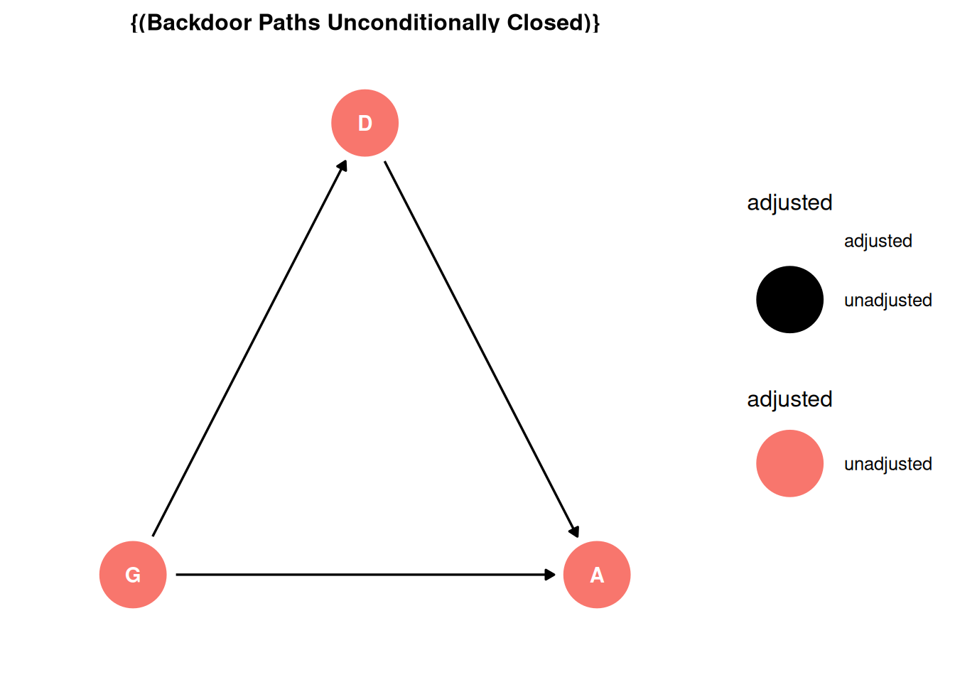
Prior predictive simulation
# Load data
tar_load(grants)

# Print priors used
tar_read(h05_q01_brms_prior)
prior class coef group resp dpar nlpar lb ub source
normal(0, 1) Intercept <NA> <NA> user
normal(0, 0.5) b <NA> <NA> user# Load model
tar_load(h05_q01_brms_sample_prior)
h05_q01_brms_sample_prior Family: binomial
Links: mu = logit
Formula: awards | trials(applications) ~ gender
Data: h05_q01_brms_data (Number of observations: 18)
Draws: 4 chains, each with iter = 2000; warmup = 1000; thin = 1;
total post-warmup draws = 4000
Regression Coefficients:
Estimate Est.Error l-95% CI u-95% CI Rhat Bulk_ESS Tail_ESS
Intercept -0.00 1.00 -2.01 1.99 1.00 3858 2964
genderm 0.01 0.50 -0.98 1.01 1.00 3643 2569
Draws were sampled using sample(hmc). For each parameter, Bulk_ESS
and Tail_ESS are effective sample size measures, and Rhat is the potential
scale reduction factor on split chains (at convergence, Rhat = 1).# Read N draws from the priors and append expected predictions
n_draws <- 100
q01_pred_prior <- h05_q01_brms_sample_prior |>
add_predicted_draws(newdata = grants, ndraws = n_draws)
# Plot prior expectations for acceptance rate and gender
ggplot(q01_pred_prior) +
stat_halfeye(aes(.prediction / applications, gender), alpha = 0.5) +
labs(x = 'Predicted acceptance rate', y = 'Gender') +
xlim(0, 1)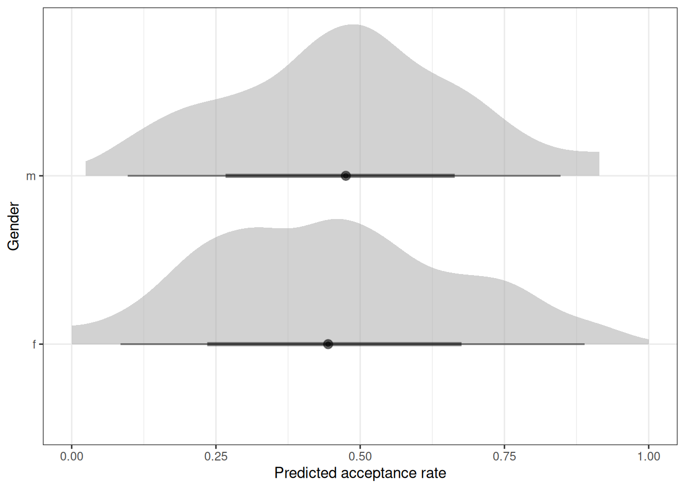
# Compare estimates between gender
setDT(q01_pred_prior)
q01_pred_prior[, est := .prediction / applications]
q01_pred_prior_compare <- dcast(
    q01_pred_prior,
    .draw + discipline ~ gender,
    value.var = 'est'
)

# Plot prior expectations comparing gender
ggplot(q01_pred_prior_compare) +
    geom_density2d_filled(aes(f, m)) +
    labs(x = 'F', y = 'M') +
    scale_fill_viridis_d() +
    coord_equal()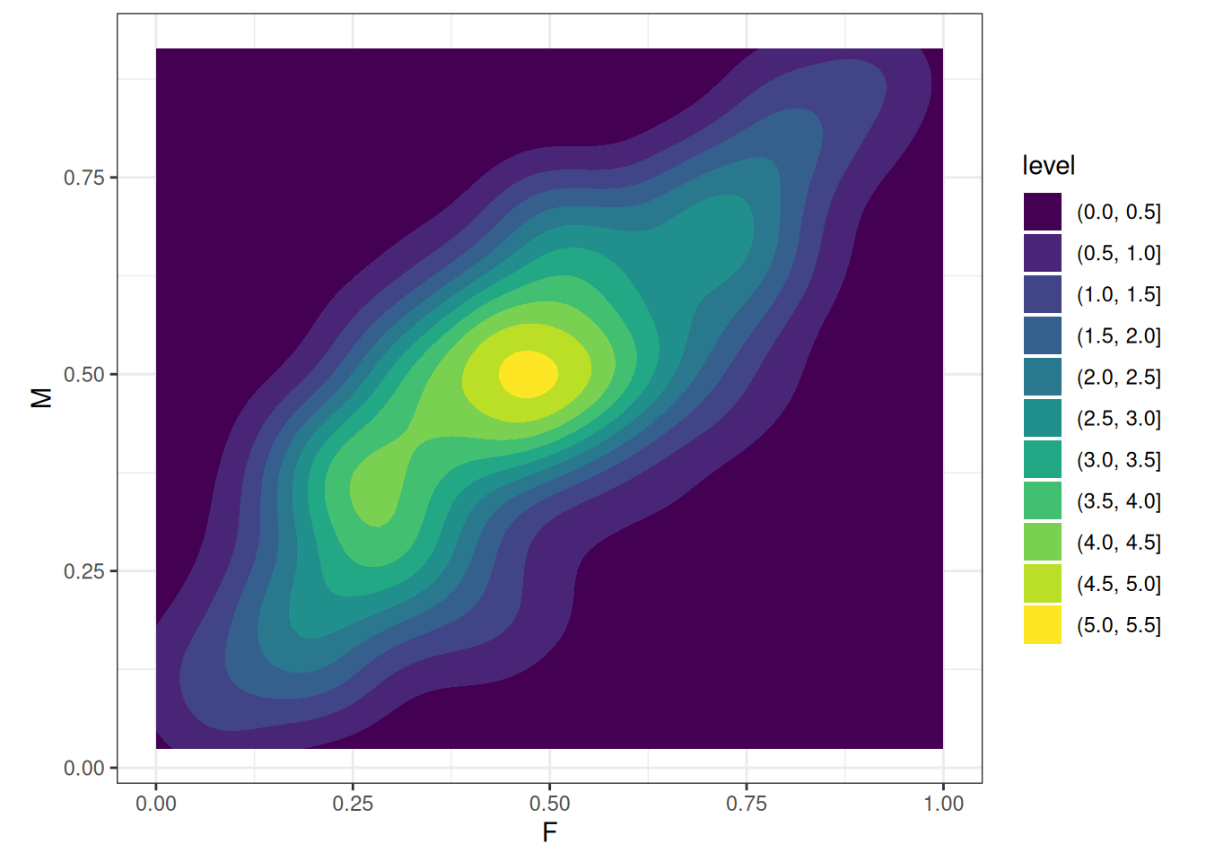
Analyze the data
# Load model
tar_load(h05_q01_brms_sample)
h05_q01_brms_sample
Family: binomial
Links: mu = logit
Formula: awards | trials(applications) ~ gender
Data: h05_q01_brms_data (Number of observations: 18)
Draws: 4 chains, each with iter = 2000; warmup = 1000; thin = 1;
total post-warmup draws = 4000
Regression Coefficients:
Estimate Est.Error l-95% CI u-95% CI Rhat Bulk_ESS Tail_ESS
Intercept -1.73 0.08 -1.89 -1.58 1.00 2114 2527
genderm 0.20 0.10 0.00 0.40 1.00 2483 2606
Draws were sampled using sample(hmc). For each parameter, Bulk_ESS
and Tail_ESS are effective sample size measures, and Rhat is the potential
scale reduction factor on split chains (at convergence, Rhat = 1).n_draws <- 100
q01_pred <- h05_q01_brms_sample |>
add_predicted_draws(newdata = grants, ndraws = n_draws)
# Plot expectations for acceptance rate and gender
ggplot(q01_pred) +
stat_halfeye(aes(.prediction / applications, gender), alpha = 0.5) +
labs(x = 'Predicted acceptance rate', y = 'Gender') +
xlim(0, 1)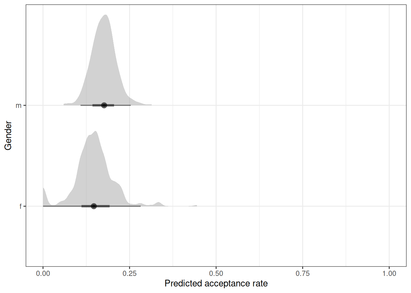
# Estimated marginal effects
marg_eff <- emmeans(h05_q01_brms_sample, ~gender, regrid = 'response')
marg_eff
gender prob lower.HPD upper.HPD
f 0.150 0.130 0.171
m 0.177 0.159 0.197
Point estimate displayed: median
HPD interval probability: 0.95 contrast(marg_eff, method = 'pairwise') contrast estimate lower.HPD upper.HPD
f - m -0.027 -0.0535 -0.000329
Point estimate displayed: median
HPD interval probability: 0.95 Question 2
Now estimate the DIRECT causal effect of gender on grant awards. Use the same DAG as above to justify one or more binomial models. Compute the average direct causal effect of gender, weighting each discipline in proportion to the number of applications in the sample. Refer to the marginal effect example in Lecture 9 for help
Estimand
What is the average direct causal effect of gender on grant awards, weighting each discipline in proportion to the number of applications in the sample.
Scientific model
dag <- dagify(
    D ~ G,
    A ~ G + D,
  coords = coords,
    exposure = 'G',
    outcome = 'A'
)
ggdag_status(dag, seed = 2, layout = 'auto') + theme_dag()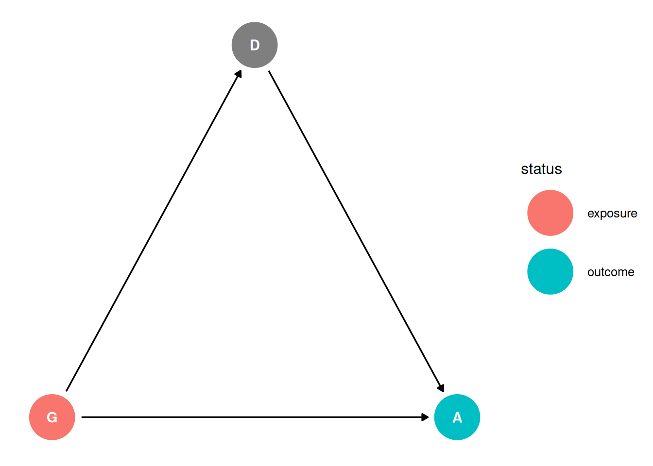
Backdoor criterion
- Identify all paths connecting treatment to the outcome, regardless of the direction of arrows
G -> AG -> D -> A
- Identify paths with arrows entering the treatment (backdoor). These are non-casual paths, because causal paths exit the treatment (frontdoor).
G -> AG -> D -> A
- Find adjustment sets that close all backdoor/non-causal paths.
There are no backdoor paths entering the treatment (G). There is a direct path from G -> A and an indirect path through D. The adjustment set for the direct effect includes D.
ggdag_adjustment_set(dag, effect = 'direct') + theme_dag()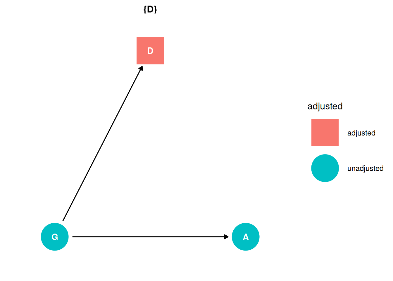
Prior predictive simulation
# Load model
tar_load(h05_q02_brms_sample_prior)
h05_q02_brms_sample_prior
Family: binomial
Links: mu = logit
Formula: awards | trials(applications) ~ gender * discipline
Data: h05_q02_brms_data (Number of observations: 18)
Draws: 4 chains, each with iter = 2000; warmup = 1000; thin = 1;
total post-warmup draws = 4000
Regression Coefficients:
Estimate Est.Error l-95% CI u-95% CI Rhat
Intercept 0.00 1.06 -2.09 2.07 1.00
genderm 0.00 0.50 -0.95 0.95 1.00
disciplineEarthDlifesciences -0.00 0.52 -1.05 1.02 1.00
disciplineHumanities 0.01 0.49 -0.93 0.94 1.00
disciplineInterdisciplinary 0.00 0.49 -0.96 1.01 1.00
disciplineMedicalsciences 0.01 0.50 -0.94 0.97 1.00
disciplinePhysicalsciences -0.00 0.51 -0.98 0.99 1.00
disciplinePhysics 0.00 0.51 -0.99 1.01 1.00
disciplineSocialsciences 0.00 0.50 -0.97 1.01 1.00
disciplineTechnicalsciences 0.00 0.51 -0.99 1.00 1.00
genderm:disciplineEarthDlifesciences 0.01 0.50 -1.00 0.95 1.00
genderm:disciplineHumanities 0.00 0.49 -0.96 0.96 1.00
genderm:disciplineInterdisciplinary -0.00 0.50 -0.98 0.98 1.00
genderm:disciplineMedicalsciences -0.00 0.50 -0.95 0.99 1.00
genderm:disciplinePhysicalsciences 0.00 0.50 -0.98 0.99 1.00
genderm:disciplinePhysics 0.00 0.51 -0.98 0.98 1.00
genderm:disciplineSocialsciences -0.01 0.50 -0.97 0.97 1.00
genderm:disciplineTechnicalsciences 0.00 0.50 -0.96 0.96 1.00
Bulk_ESS Tail_ESS
Intercept 11228 2475
genderm 9845 2663
disciplineEarthDlifesciences 10617 2589
disciplineHumanities 9419 3312
disciplineInterdisciplinary 11409 2718
disciplineMedicalsciences 10392 2855
disciplinePhysicalsciences 10511 2837
disciplinePhysics 9824 3004
disciplineSocialsciences 9013 2758
disciplineTechnicalsciences 8923 2950
genderm:disciplineEarthDlifesciences 9274 2878
genderm:disciplineHumanities 11488 2844
genderm:disciplineInterdisciplinary 11526 3056
genderm:disciplineMedicalsciences 11500 3027
genderm:disciplinePhysicalsciences 10995 3004
genderm:disciplinePhysics 9661 2723
genderm:disciplineSocialsciences 8546 2821
genderm:disciplineTechnicalsciences 10627 2889
Draws were sampled using sample(hmc). For each parameter, Bulk_ESS
and Tail_ESS are effective sample size measures, and Rhat is the potential
scale reduction factor on split chains (at convergence, Rhat = 1).n_draws <- 100
q02_pred_prior <- h05_q02_brms_sample_prior |>
add_predicted_draws(newdata = grants, ndraws = n_draws)
# Plot prior expectations for acceptance rate and gender
ggplot(q02_pred_prior) +
stat_halfeye(aes(.prediction / applications, gender), alpha = 0.5) +
labs(x = 'Predicted acceptance rate', y = 'Gender') +
facet_wrap(~discipline) +
xlim(0, 1)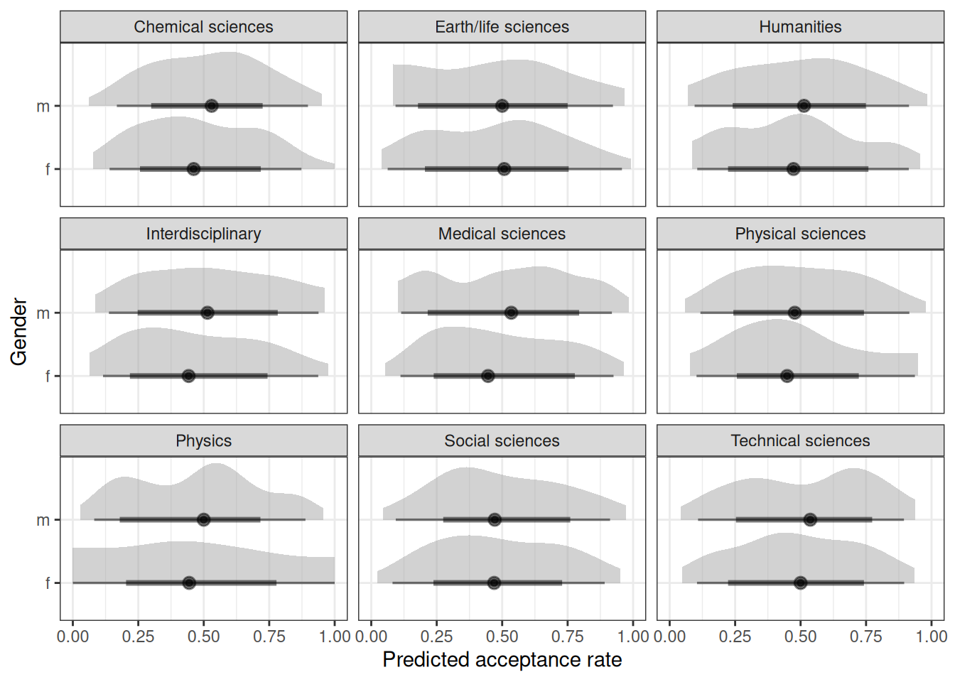
# Compare estimates between gender
setDT(q02_pred_prior)
q02_pred_prior[, est := .prediction / applications]
q02_pred_prior_compare <- dcast(
    q02_pred_prior,
    .draw + discipline ~ gender,
    value.var = 'est'
)

# Plot prior expectations comparing gender
ggplot(q02_pred_prior_compare) +
    geom_density2d_filled(aes(f, m)) +
    labs(x = 'F', y = 'M') +
    facet_wrap(~ discipline) +
    scale_fill_viridis_d() +
    coord_equal()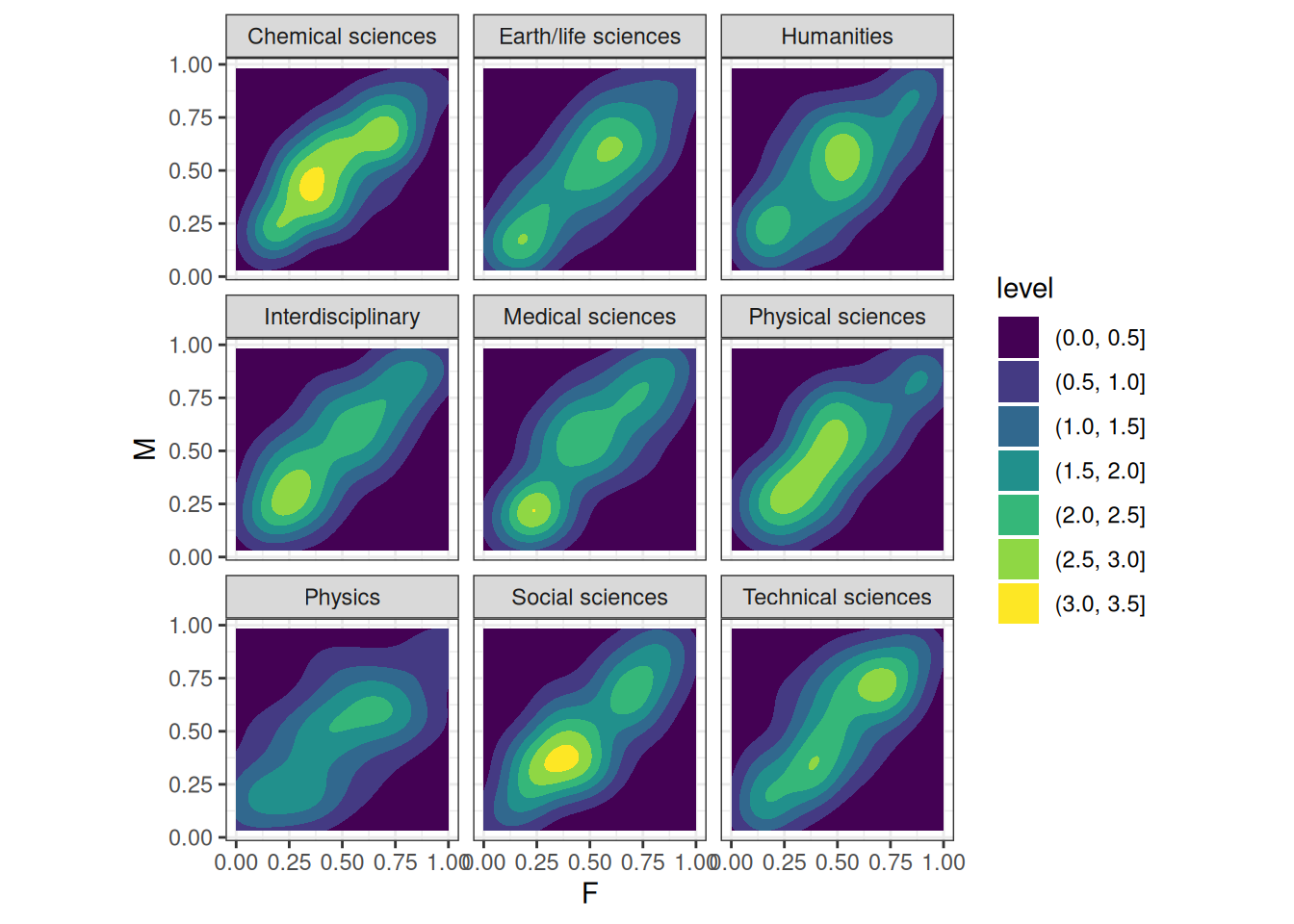
Analyze the data
data_grantsfunction() {
data("NWOGrants")
DT <- data.table(NWOGrants)
DT[, index_gender := .GRP, gender]
DT[, index_discipline := .GRP, discipline]
DT[, gender := factor(gender)]
DT[, discipline := factor(discipline)]
return(DT)
}# Load model
tar_load(h05_q02_brms_sample)
h05_q02_brms_sample Family: binomial
Links: mu = logit
Formula: awards | trials(applications) ~ gender * discipline
Data: h05_q02_brms_data (Number of observations: 18)
Draws: 4 chains, each with iter = 2000; warmup = 1000; thin = 1;
total post-warmup draws = 4000
Regression Coefficients:
Estimate Est.Error l-95% CI u-95% CI Rhat
Intercept -1.40 0.16 -1.72 -1.08 1.00
genderm 0.15 0.17 -0.18 0.49 1.00
disciplineEarthDlifesciences -0.26 0.23 -0.72 0.19 1.00
disciplineHumanities -0.09 0.22 -0.54 0.34 1.00
disciplineInterdisciplinary -0.05 0.26 -0.56 0.45 1.00
disciplineMedicalsciences -0.56 0.21 -0.98 -0.15 1.00
disciplinePhysicalsciences 0.05 0.29 -0.53 0.61 1.00
disciplinePhysics 0.12 0.35 -0.55 0.79 1.00
disciplineSocialsciences -0.58 0.20 -0.97 -0.20 1.00
disciplineTechnicalsciences -0.06 0.27 -0.60 0.45 1.00
genderm:disciplineEarthDlifesciences 0.32 0.27 -0.21 0.85 1.00
genderm:disciplineHumanities -0.40 0.27 -0.93 0.12 1.00
genderm:disciplineInterdisciplinary -0.57 0.32 -1.18 0.05 1.00
genderm:disciplineMedicalsciences 0.30 0.26 -0.21 0.82 1.00
genderm:disciplinePhysicalsciences -0.20 0.32 -0.83 0.43 1.00
genderm:disciplinePhysics 0.08 0.37 -0.64 0.82 1.00
genderm:disciplineSocialsciences 0.10 0.23 -0.35 0.55 1.00
genderm:disciplineTechnicalsciences -0.32 0.30 -0.90 0.26 1.00
Bulk_ESS Tail_ESS
Intercept 3249 3111
genderm 3497 3275
disciplineEarthDlifesciences 4760 3243
disciplineHumanities 3830 3090
disciplineInterdisciplinary 4425 2806
disciplineMedicalsciences 3708 2927
disciplinePhysicalsciences 4912 3060
disciplinePhysics 5213 3105
disciplineSocialsciences 3525 3142
disciplineTechnicalsciences 4493 3441
genderm:disciplineEarthDlifesciences 5090 3240
genderm:disciplineHumanities 4836 3415
genderm:disciplineInterdisciplinary 5436 3254
genderm:disciplineMedicalsciences 4480 3016
genderm:disciplinePhysicalsciences 5308 3218
genderm:disciplinePhysics 5238 3223
genderm:disciplineSocialsciences 3968 3279
genderm:disciplineTechnicalsciences 4531 2963
Draws were sampled using sample(hmc). For each parameter, Bulk_ESS
and Tail_ESS are effective sample size measures, and Rhat is the potential
scale reduction factor on split chains (at convergence, Rhat = 1).# Read N draws from the priors and append expected predictions
n_draws <- 100
q02_pred <- h05_q02_brms_sample |>
add_predicted_draws(newdata = grants, ndraws = n_draws)
# Plot expectations for acceptance rate and gender
ggplot(q02_pred) +
stat_halfeye(aes(.prediction / applications, gender), alpha = 0.5) +
labs(x = 'Predicted acceptance rate', y = 'Gender') +
facet_wrap(~discipline) +
xlim(0, 1)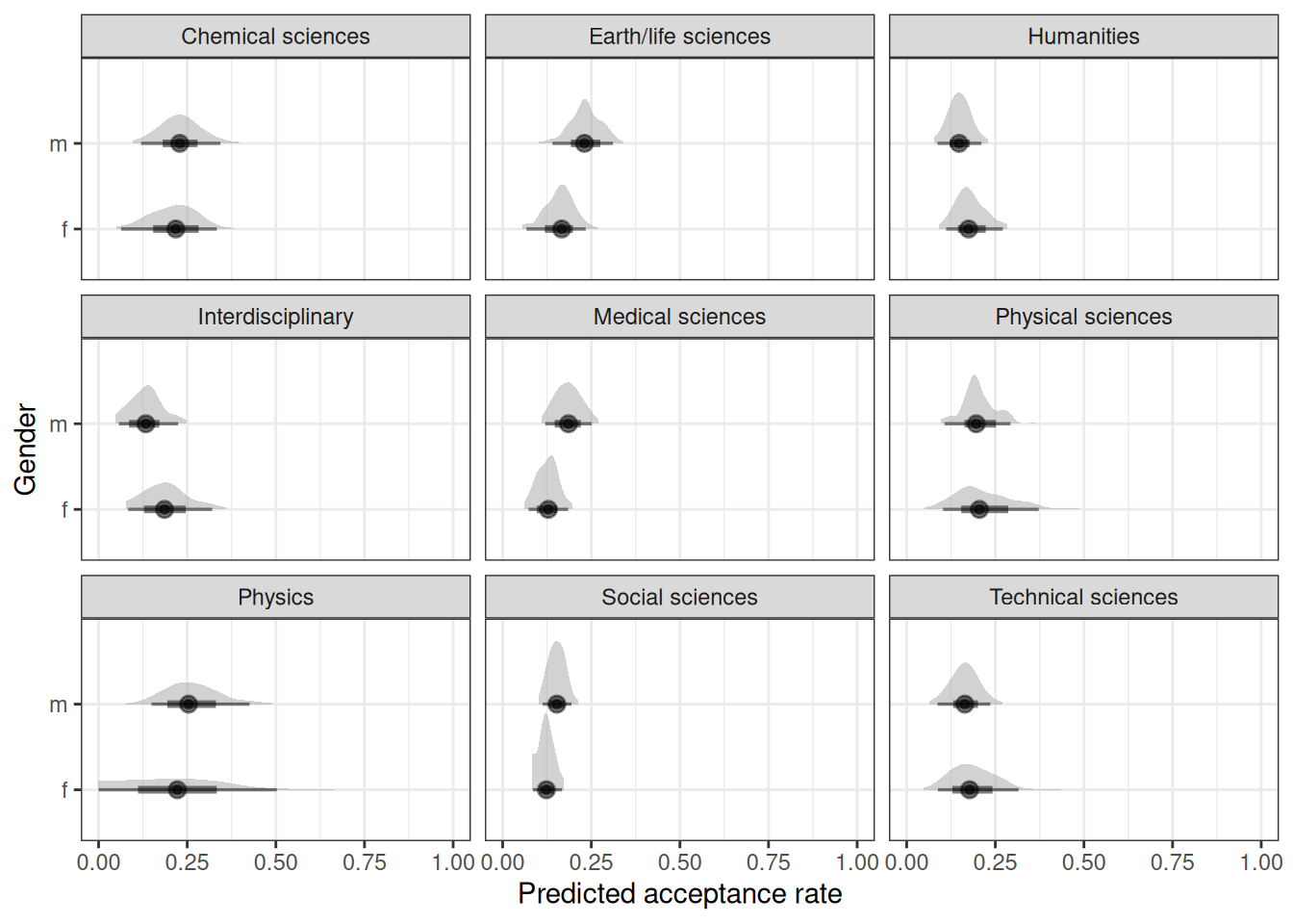
# Estimated marginal effects
marg_eff <- emmeans(
    h05_q02_brms_sample,
    ~ gender | discipline,
    regrid = 'response'
)
marg_eff
discipline = Chemical sciences:
gender prob lower.HPD upper.HPD
f 0.198 0.1464 0.246
m 0.223 0.1713 0.290
discipline = Earth/life sciences:
gender prob lower.HPD upper.HPD
f 0.160 0.1101 0.214
m 0.235 0.1733 0.296
discipline = Humanities:
gender prob lower.HPD upper.HPD
f 0.185 0.1345 0.239
m 0.150 0.1106 0.196
discipline = Interdisciplinary:
gender prob lower.HPD upper.HPD
f 0.190 0.1276 0.263
m 0.135 0.0818 0.196
discipline = Medical sciences:
gender prob lower.HPD upper.HPD
f 0.124 0.0892 0.161
m 0.182 0.1390 0.229
discipline = Physical sciences:
gender prob lower.HPD upper.HPD
f 0.206 0.1253 0.302
m 0.198 0.1344 0.261
discipline = Physics:
gender prob lower.HPD upper.HPD
f 0.218 0.1197 0.350
m 0.262 0.1648 0.363
discipline = Social sciences:
gender prob lower.HPD upper.HPD
f 0.121 0.0923 0.152
m 0.151 0.1190 0.186
discipline = Technical sciences:
gender prob lower.HPD upper.HPD
f 0.190 0.1236 0.268
m 0.165 0.1165 0.213
Point estimate displayed: median
HPD interval probability: 0.95 contrast(marg_eff, method = 'pairwise')discipline = Chemical sciences:
contrast estimate lower.HPD upper.HPD
f - m -0.02560 -0.0838 0.02854
discipline = Earth/life sciences:
contrast estimate lower.HPD upper.HPD
f - m -0.07411 -0.1475 0.00622
discipline = Humanities:
contrast estimate lower.HPD upper.HPD
f - m 0.03480 -0.0332 0.09829
discipline = Interdisciplinary:
contrast estimate lower.HPD upper.HPD
f - m 0.05477 -0.0200 0.14052
discipline = Medical sciences:
contrast estimate lower.HPD upper.HPD
f - m -0.05733 -0.1161 -0.00242
discipline = Physical sciences:
contrast estimate lower.HPD upper.HPD
f - m 0.00827 -0.0901 0.10526
discipline = Physics:
contrast estimate lower.HPD upper.HPD
f - m -0.04156 -0.1767 0.09056
discipline = Social sciences:
contrast estimate lower.HPD upper.HPD
f - m -0.02952 -0.0749 0.01170
discipline = Technical sciences:
contrast estimate lower.HPD upper.HPD
f - m 0.02449 -0.0515 0.11938
Point estimate displayed: median
HPD interval probability: 0.95 Question 3
OPTIONAL CHALLENGE. The data in data(UFClefties) are the outcomes of 205 Ultimate Fighting Championship (UFC) matches (see ?UFClefties for details). It is widely believed that left-handed fighters (aka “Southpaws”) have an advantage against right-handed fighters, and left-handed men are indeed over-represented among fighters (and fencers and tennis players) compared to the general population. Estimate the average advantage, if any, that a left-handed fighter has against right-handed fighters. Based upon your estimate, why do you think left-handers are over-represented among UFC fighters?
?UFClefties- fight: Unique identifier for match
- episode: Identifier for UFC episode
- fight.in.episode: Order of fight in episode
- fighter1.win: 1 if fighter 1 won the match; 0 if fight 2 won
- fighter1: Unique identifier for fighter 1
- fighter2: Unique identifier for fighter 2
- fighter1.lefty: 1 if fighter 1 was left handed; 0 otherwise
- fighter2.lefty: 1 if fighter 2 was left handed; 0 otherwise
Estimand
What is the direct effect of handedness on UFC match outcomes?
Analyze the data
data_ufcfunction() {
data("UFClefties")
DT <- data.table(UFClefties)
DT[fighter1.lefty == 1 & fighter2.lefty == 0,
colnames(DT) := .SD,
.SDcols = stri_replace(
colnames(DT),
regex = c('1', '2'),
replacement = c('2', '1')
)]
DT[, hand_1 := c('L', 'R')[fighter1.lefty + 1]]
DT[, hand_2 := c('L', 'R')[fighter2.lefty + 1]]
DT[, hand_pair := factor(paste(hand_1, hand_2, sep = '-'))]
DT[, .(n_fight = .N, n_win = sum(fighter1.win)), by = hand_pair]
}# Load data
tar_load(ufc)
# Load model
tar_load(h05_q03_brms_sample)
h05_q03_brms_sample Family: binomial
Links: mu = logit
Formula: n_win | trials(n_fight) ~ hand_pair
Data: h05_q03_brms_data (Number of observations: 3)
Draws: 4 chains, each with iter = 2000; warmup = 1000; thin = 1;
total post-warmup draws = 4000
Regression Coefficients:
Estimate Est.Error l-95% CI u-95% CI Rhat Bulk_ESS Tail_ESS
Intercept 0.16 0.16 -0.15 0.49 1.00 3743 3192
hand_pairLMR -0.19 0.25 -0.67 0.30 1.00 2862 2670
hand_pairRMR -0.30 0.38 -1.03 0.44 1.00 2347 2547
Draws were sampled using sample(hmc). For each parameter, Bulk_ESS
and Tail_ESS are effective sample size measures, and Rhat is the potential
scale reduction factor on split chains (at convergence, Rhat = 1).n_draws <- 100
q03_pred <- h05_q03_brms_sample |>
add_predicted_draws(newdata = ufc, ndraws = n_draws)
# Plot predicted win rate by handedness
ggplot(q03_pred) +
stat_halfeye(aes(.prediction / n_fight, hand_pair), alpha = 0.5) +
labs(x = 'Predicted win rate', y = 'Handedness') +
xlim(0, 1)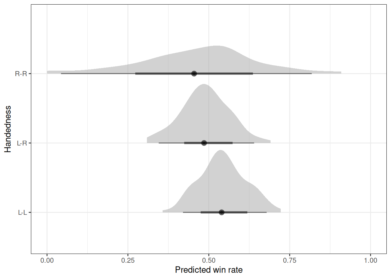
# Estimated marginal effects
marg_eff <- emmeans(h05_q03_brms_sample, ~hand_pair, regrid = 'response')
marg_eff
hand_pair prob lower.HPD upper.HPD
L-L 0.541 0.462 0.619
L-R 0.495 0.390 0.594
R-R 0.466 0.290 0.646
Point estimate displayed: median
HPD interval probability: 0.95 contrast(marg_eff) contrast estimate lower.HPD upper.HPD
(L-L) effect 0.03996 -0.0368 0.1111
(L-R) effect -0.00541 -0.1047 0.0894
(R-R) effect -0.03420 -0.1525 0.0937
Point estimate displayed: median
HPD interval probability: 0.95 Left handed fighters do not appear to have an advantage over right handed fighters.