Linear models are additive combinations of variables They can be used for many applications, the fit is ok but not ideal Using linear models gives up scientific information we could use to better inform statistical analysis
LMs, GLMs, GLMMs are flexible machines for decscribing associations
Without an external causal model, linear models have no causal interpretation
Example: height
The weight of humans is proportional to height. For example, represent humans as a cylinder.
Starting from the equation for the volume of a cylinder:
\(V = \pi r^{2} h\)
Represent the radius as proportion of height
\(V = \pi (ph)^{2} h\)
Finally, the weight depends on the density (k) of the cylinder
\(W = kV = k \pi (ph)^{2} h\)
And simplified, the formula for the expected weight is
\(W = k \pi p^{2}h^{3}\)
This is not a regression model, it is a scientific model that arises from the physical structure of human bodies.
Statistical model
\(W_{i} \sim Distribution(\mu_{i})\)
\(\mu_{i} = k \pi p^{2} h^{3}\)
\(p \sim Distribution(\)
\(k \sim Distribution()\)
Set priors: choose measurement scales and simulate.
Units:
\(\mu_{i}\): kg
\(k\): \(kg/cm^{3}\)
\(h^{3}\)
Measurement scales are social constructs, and it can be easier to divide them out. We can do that by rescaling by, eg. the mean height and weight, resulting in the same data dimensionless. By dividing by the mean, anything larger than 1 is larger than the mean, anything less than 1 is less than the mean.
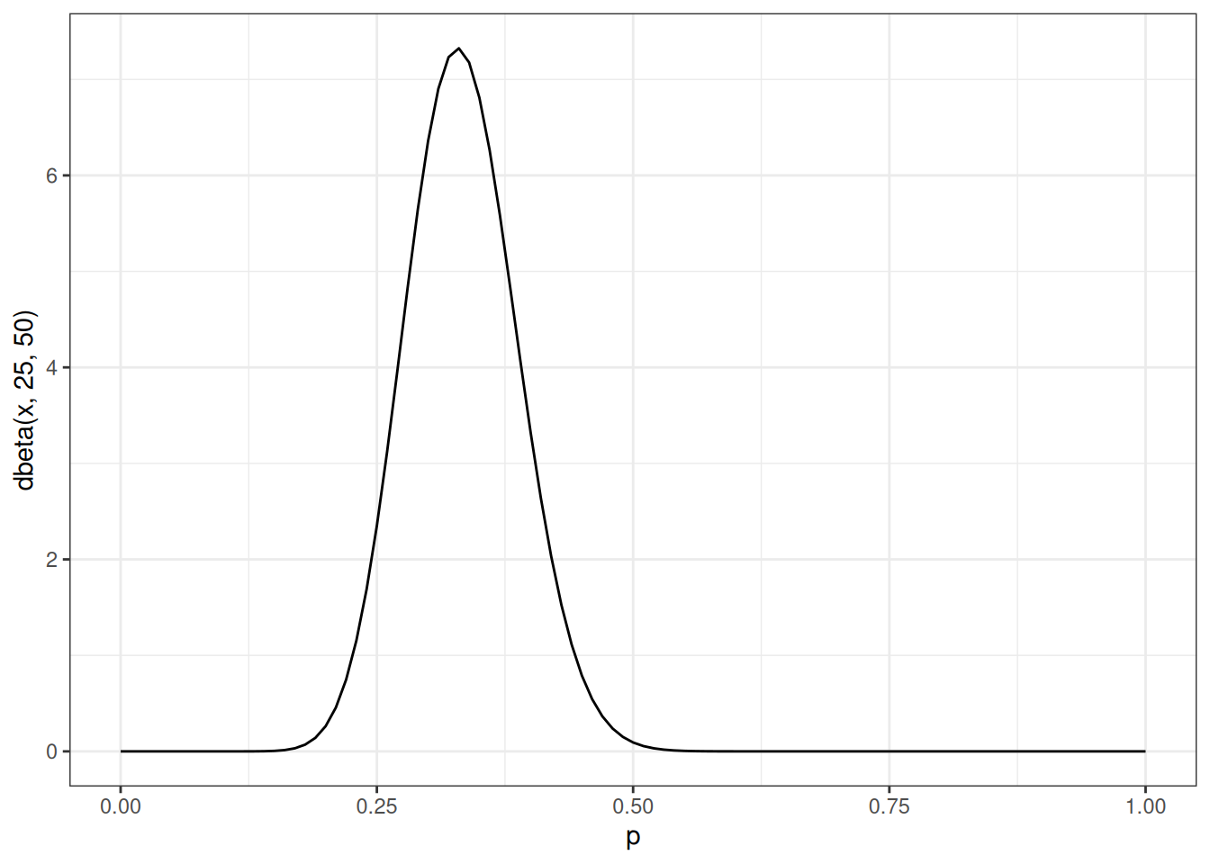
P is a proporiton, therefore between 0-1, less than 0.5 in this case because the radius of a body in this population is less than a half of its height.
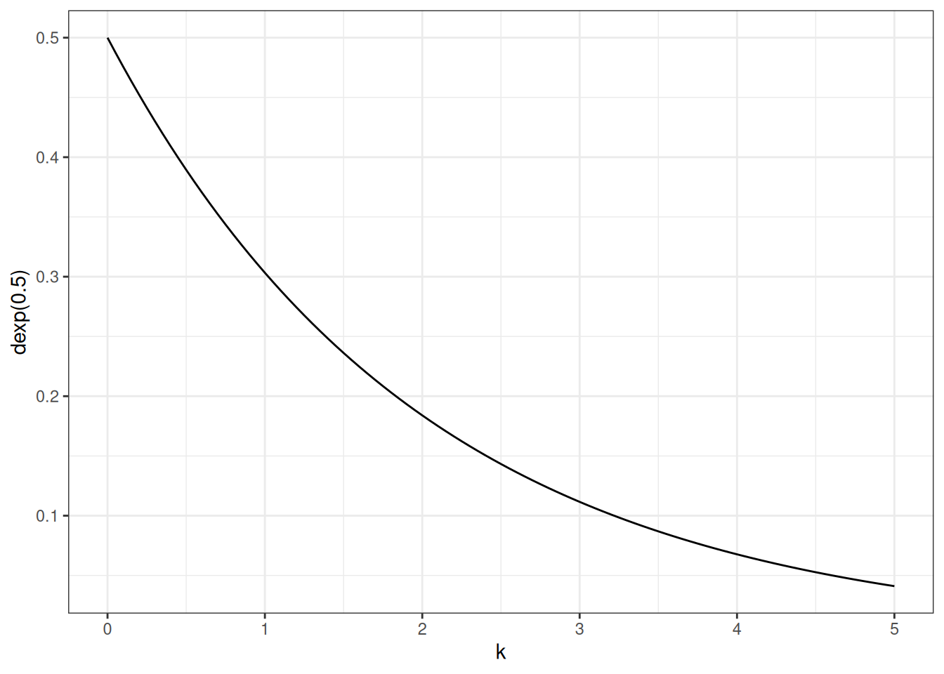
k is a density, it is a positive real number, greater than 1.
ggplot()+stat_function(fun =dexp, args =list(rate =0.5))+xlim(0, 5)+labs(x ='k', y ='dexp(0.5)')
Weight is a positive real, variance scales with the mean. Growth is multiplicative, log-normal is natural choice.
LogNormal is parameterized using the mu and sigma: mu in log-normal is mean of log, not mean of observed. Therefore when we model, we need to exponentiate mu because the formula corresponds to weight on the natural scale.
\(W_{i} \sim LogNormal(\mu_{i}, \sigma)\)
\(exp(\mu_{i}) = k \pi p^{2} h^{3}\)
\(p \sim Beta(25, 50)\)
\(k \sim Exponential(0.5)\)
\(\sigma \sim Exponential(1)\)
DT<-data_Howell()form<-bf(scale_weight_div_mean~log(k*3.1415*p^2*scale_height_div_mean^3),p~1,k~1, nl =TRUE)get_prior(form, data =DT, family ='lognormal')
                prior class      coef group resp dpar nlpar lb ub       source
 student_t(3, 0, 2.5) sigma                                  0         default
               (flat)     b                               k            default
               (flat)     b Intercept                     k       (vectorized)
               (flat)     b                               p            default
               (flat)     b Intercept                     p       (vectorized)
tar_load(m_l19_nl_howell)m_l19_nl_howell$prior
            prior class      coef group resp dpar nlpar lb ub       source
 exponential(0.5)     b                               k  0            user
 exponential(0.5)     b Intercept                     k  0    (vectorized)
     beta(25, 50)     b                               p  0  1         user
     beta(25, 50)     b Intercept                     p  0  1 (vectorized)
   exponential(1) sigma                                  0            user
m_l19_nl_howell
 Family: lognormal
  Links: mu = identity; sigma = identity
Formula: scale_weight_div_mean ~ log(k * 3.1415 * p^2 * scale_height_div_mean^3)
         p ~ 1
         k ~ 1
   Data: data_Howell() (Number of observations: 544)
  Draws: 4 chains, each with iter = 2000; warmup = 1000; thin = 1;
         total post-warmup draws = 4000

Population-Level Effects:
            Estimate Est.Error l-95% CI u-95% CI Rhat Bulk_ESS Tail_ESS
p_Intercept     0.34      0.05     0.25     0.45 1.00      831     1008
k_Intercept     2.80      0.87     1.52     4.95 1.00      832     1047

Family Specific Parameters:
      Estimate Est.Error l-95% CI u-95% CI Rhat Bulk_ESS Tail_ESS
sigma     0.21      0.01     0.19     0.22 1.00     1415     1252

Draws were sampled using sampling(NUTS). For each parameter, Bulk_ESS
and Tail_ESS are effective sample size measures, and Rhat is the potential
scale reduction factor on split chains (at convergence, Rhat = 1).
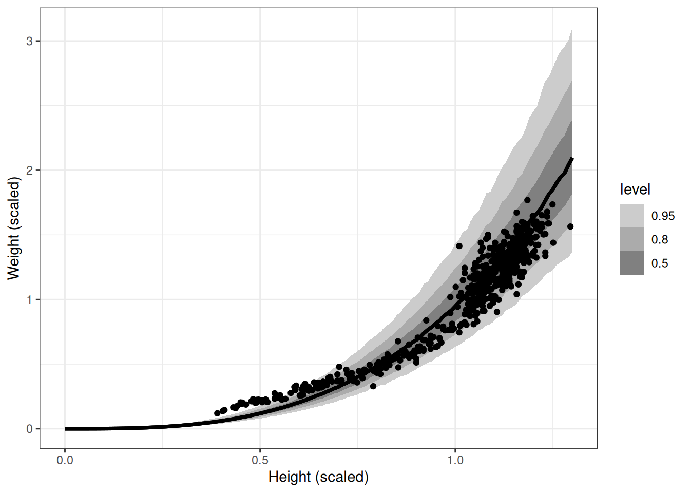
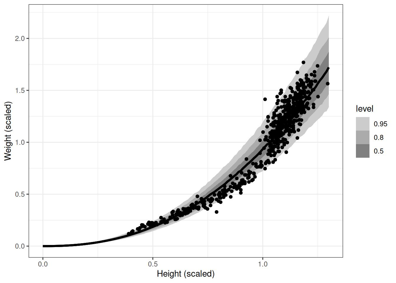
pred<-add_predicted_draws(m_l19_nl_howell, newdata =data.frame(scale_height_div_mean =seq(0, 1.3, 0.01)))ggplot(pred, aes(scale_height_div_mean, .prediction))+stat_lineribbon()+geom_point(aes(scale_height_div_mean, scale_weight_div_mean), data =DT)+scale_fill_grey(start =0.8, end =0.5)+labs(x ='Height (scaled)', y ='Weight (scaled)')
Models using scientific structure can be easier to tune, because differences from prediction error are more closely tied to the problem at hand, rather than geocentric type models.
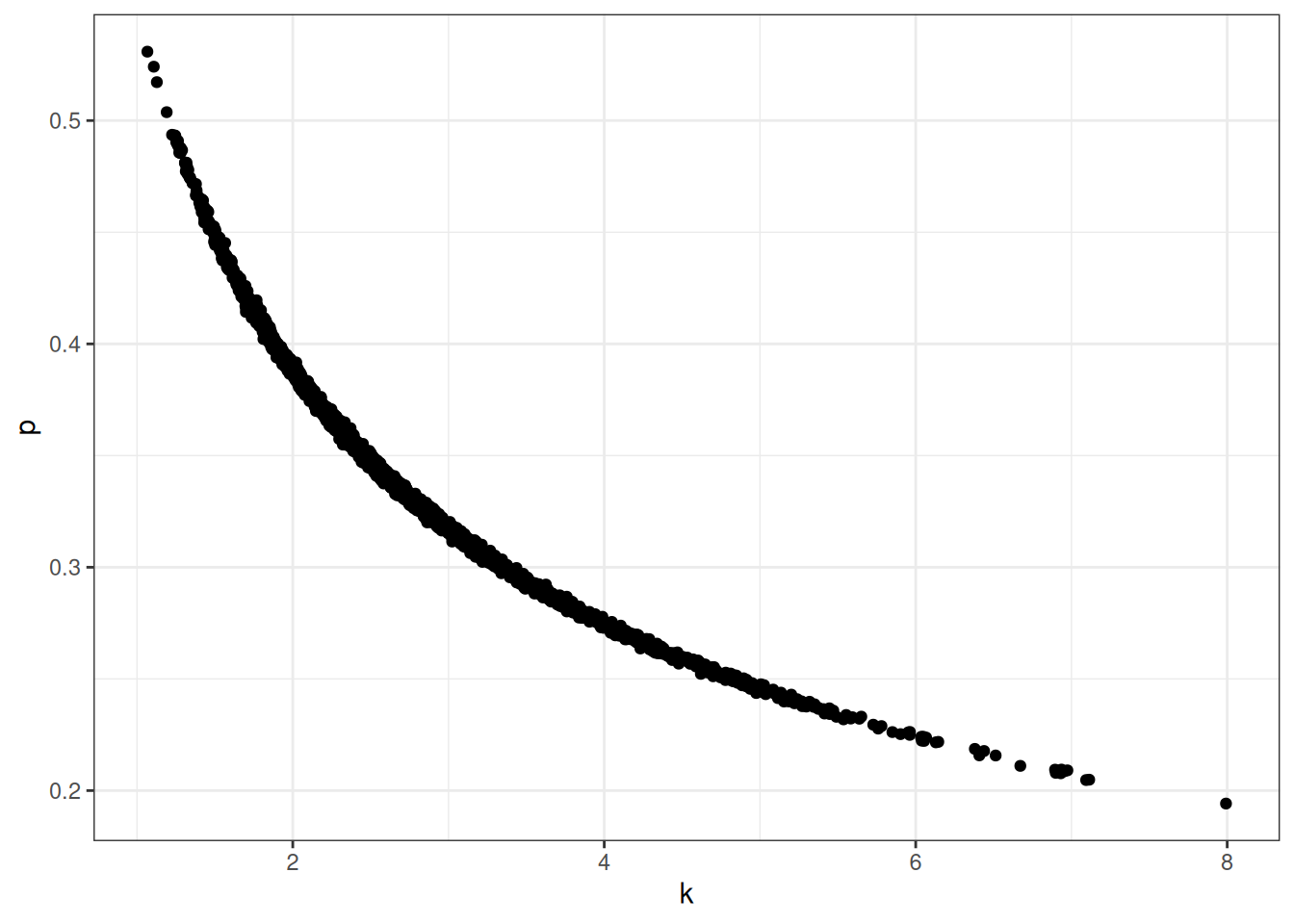
The posterior shows that the relationship between k and p is a negative curve where as k increases the values for p decrease. The model has identified a mathematical function in our formula, that could be used directly instead of including these parameters in the model.
ggplot(as_draws_df(m_l19_nl_howell))+geom_point(aes(b_k_Intercept, b_p_Intercept))+labs(x ='k', y ='p')
Taking an example individual with scaled height = 1 and scaled weight = 1, we can solve for k.
\(\mu_{i} = k \pi p^{2} h^{3}\)
\((1) = k \pi p^{2} (1)^{3}\)
\(k = \frac{1}{\pi p^{2}}\)
This is the relationship show in the graph above.
Further, given:
\((1) = k \pi p^{2} (1)^{3}\)
Subbing in the expression for k above, we get:
\((1) = \pi \theta (1)^{3}\)
\(\theta\) is used to represent \(k p^2\) and therefore it must be
\(\theta \approx \pi^{-1}\)
Given this, there are no parameters in the model, it is dimensionless. Restructuring the model without those two fparameters, the model returns the same result and, as a bonus, fits much more efficiently.
                  prior     class                       coef group resp dpar
                 (flat)         b
                 (flat)         b logscale_height_div_meanE3
 student_t(3, 0.1, 2.5) Intercept
         exponential(1)     sigma
 nlpar lb ub       source
                  default
             (vectorized)
                  default
        0            user
m_l19_nl_howell_no_dim
 Family: lognormal
  Links: mu = identity; sigma = identity
Formula: scale_weight_div_mean ~ log(scale_height_div_mean^3)
   Data: data_Howell() (Number of observations: 544)
  Draws: 4 chains, each with iter = 2000; warmup = 1000; thin = 1;
         total post-warmup draws = 4000

Population-Level Effects:
                           Estimate Est.Error l-95% CI u-95% CI Rhat Bulk_ESS
Intercept                     -0.07      0.01    -0.08    -0.06 1.00     4665
logscale_height_div_meanE3     0.77      0.01     0.76     0.79 1.00     3452
                           Tail_ESS
Intercept                      2970
logscale_height_div_meanE3     2316

Family Specific Parameters:
      Estimate Est.Error l-95% CI u-95% CI Rhat Bulk_ESS Tail_ESS
sigma     0.13      0.00     0.12     0.13 1.00     3216     2569

Draws were sampled using sampling(NUTS). For each parameter, Bulk_ESS
and Tail_ESS are effective sample size measures, and Rhat is the potential
scale reduction factor on split chains (at convergence, Rhat = 1).
pred_no_dim<-add_predicted_draws(m_l19_nl_howell_no_dim, newdata =data.frame(scale_height_div_mean =seq(0, 1.3, 0.01)))ggplot(pred_no_dim, aes(scale_height_div_mean, .prediction))+stat_lineribbon()+geom_point(aes(scale_height_div_mean, scale_weight_div_mean), data =DT)+scale_fill_grey(start =0.8, end =0.5)+labs(x ='Height (scaled)', y ='Weight (scaled)')
State-based models
What we want is a latent state but what we have is only emissions or behaviours of a latent variable. A misguided approach would be to just analyse this data as if it is a categorical variable, disregarding the difference between the behaviour and the underlying latent state.
This family of models if common in movement, learning, population dynamics, international relations, family planning.
Example: social conformity
Do children copy the majority?
We can’t see the strategy selected, we can only see the choice.
Majority choice is consistent with many strategies:
random color would follow majority 1/3 the time
random demonstrator would follow majority 3/4 the time
random demonstration would follow majority 1/2 the time
Total evidence for majority choice is exaggerated because multiple processes lead to the majority choice beyond a majority preference.
Strategy space:
Majority
Minority
Maverick (unchosen)
Random color (ignore demonstrators)
Follow first (copy the first demonstrator)
This is a state based model. There are three possible observations: unchosen, majority or minority.