p <- seq(0, 1, 0.01)

ggplot(data.table(logit_p= logit(p), p = p)) + geom_line(aes(logit_p, p))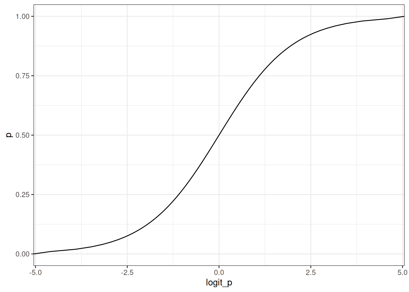
Like tide prediction engines (analog computers), the gears inside the machine bear no resemble to the observable predictions that they put out.
Linear models: expected value is an additive linear combination of parameters. Can only do this with the normal distribution because it is unbounded.
Other events are bounded. For example, probability of events are restricted to 0-1.
Generalized linear models: expected value is some function of an additive combination of parameters.
\(Y_{i} \sim Bernoulli(p_{i})\)
\(f(p_{i}) = \alpha + \beta_{{X}} X_{i} + \beta_{Z} Z_{i}\)
\(f\) is the link function
\(f(p_{i} = \alpha + \beta_{{X}} X_{i} + \beta_{Z} Z_{i})\)
\(f^{-1}\) is the inverse link function.
\(p_{i} = f^{-1}(\alpha + \beta_{{X}} X_{i} + \beta_{Z} Z_{i})\)
Logistic regression: binary [0,1] outcome and logit link, with Bernoulli distribution
Binomial regression: count [0, N] outcome and logit link, with Binomial distribution (Binomimal variables are sums of Bernoulli variables)
The distribution is matched to constraints on observed variables and the link function is matched to this distribution.
Distribution you want to use to model an observed variable is governed by the constraints on observation. Eg. you can’t have negative counts. You can’t use some test to decide if your data are “Normal”.
Bernoulli and binomial models most often use the logit link.
\(logit\) is the link function
\(logit(p_{i} = \alpha + \beta_{{X}} X_{i} + \beta_{Z} Z_{i})\)
\(logit^{-1}\) (logistic) is the inverse link function.
\(p_{i} = logit^{-1}(\alpha + \beta_{{X}} X_{i} + \beta_{Z} Z_{i})\)
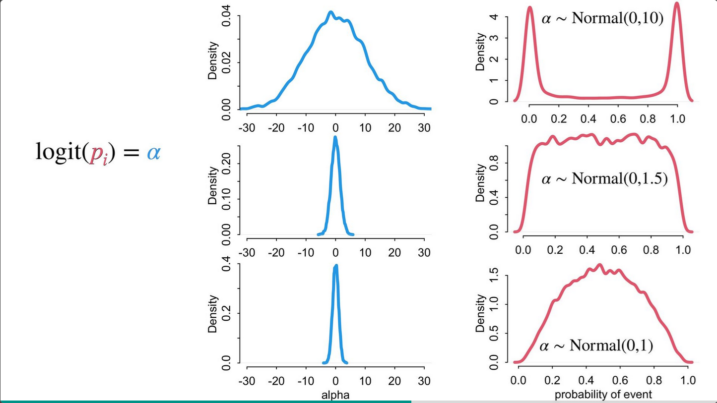
Logit link is a harsh transformation
p <- seq(0, 1, 0.01)
ggplot(data.table(logit_p= logit(p), p = p)) + geom_line(aes(logit_p, p))
The logit link compresses parameter distributions. Anything above +4 = almost always, anything below -4 = almost never.
See more here:
Traag, V.A. and Waltman, L., 2022. Causal foundations of bias, disparity and fairness. arXiv preprint arXiv:2207.13665.
suppressPackageStartupMessages(library(ggdag))
coords <- data.frame(
    name = c('G', 'D', 'A', 'G_star', 'R', 'U'),
    x =    c(1,    2,   3,   2,         4,   4),
    y =    c(0,    1,   0,  -1,        -1,   1)
)
Was there gender discrimination in graduate admissions?
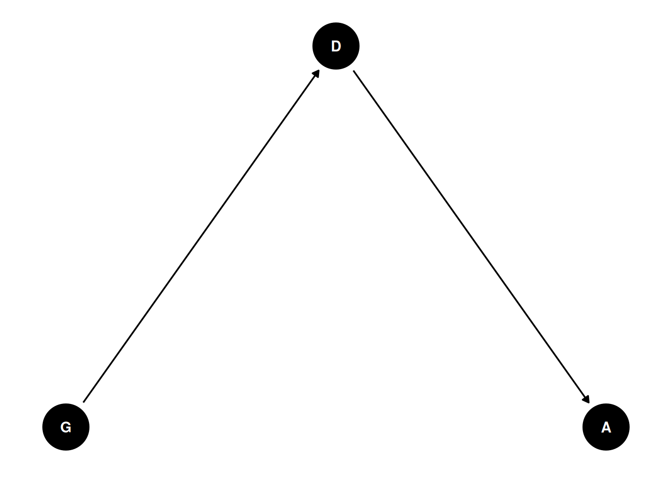
Typically, department is considered a mediating variable
What can the “causal effect of gender” mean?
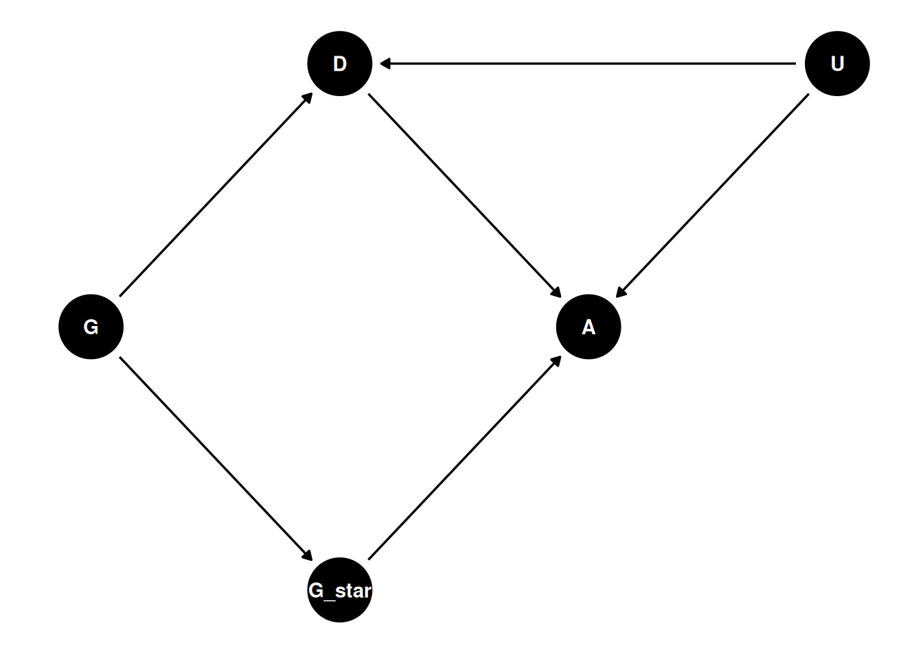
dagify(
    A ~ R + G_star + D,
    G_star ~ G,
    D ~ G,
  coords = coords
) |> ggdag(seed = 2, layout = 'auto') + theme_dag()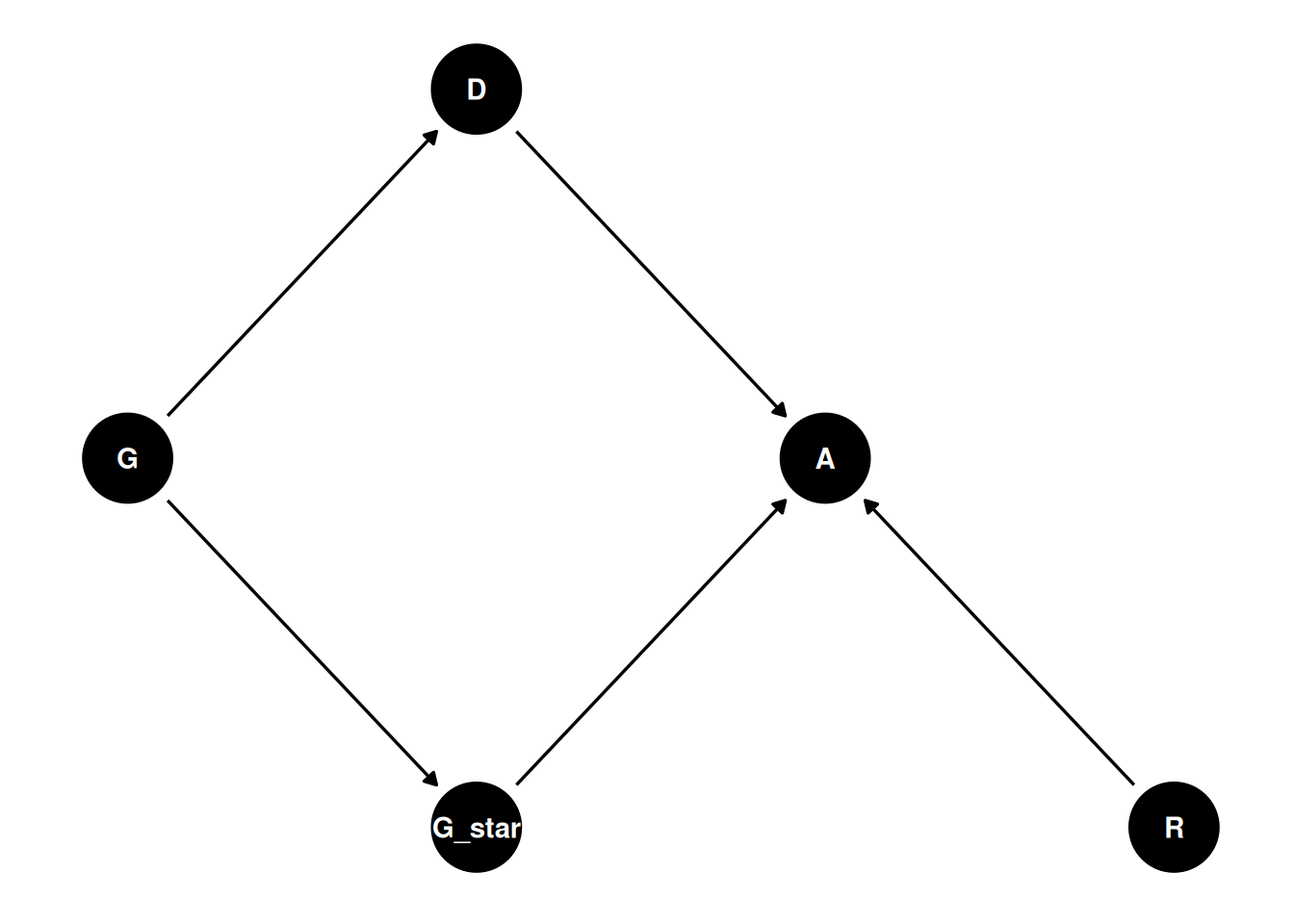
Which path represents “discrimination”?
For now, we will ignore the unobserved confounds between the mediator and the outcome.
Changing the acceptance rate where acceptance differs by department and gender, pattern of differences in acceptance rates is the same in this simulated data. This illustrates the fundamental problem of determining if discrimination is occuring.
Generative model could be greatly improved:
Total causal effect of G
\(A_{i} \sim Bernoulli(p_{i})\)
\(logit(p_{i}) = \alpha[G_{i}]\)
\(\alpha = [\alpha_{1}, \alpha_{2}]\)
Direct causal effect of G
\(A_{i} \sim Bernoulli(p_{i})\)
\(logit(p_{i}) = \alpha[G_{i}, D_{i}]\)
\(\alpha = \begin{bmatrix} \alpha_{1, 1} & \alpha_{1, 2} \\ \alpha_{2, 1} & \alpha_{2, 2}\end{bmatrix}\)
Use inverse logit function to transform variables back on probability scale. Determine if known parameters are recovered by the model.
To use a binomial distribution, aggregate the long format data into acceptance sums for each gender and department. This is equivalent to using the original data with a Bernoulli distribution.
Back to the question: what’s the average direct effect of gender across departments?
This depends on the perception of gender on the admission officer
dagify(
    A ~ G_star + D,
    G_star ~ G,
    D ~ G,
  coords = coords
) |> ggdag(seed = 2, layout = 'auto') + theme_dag()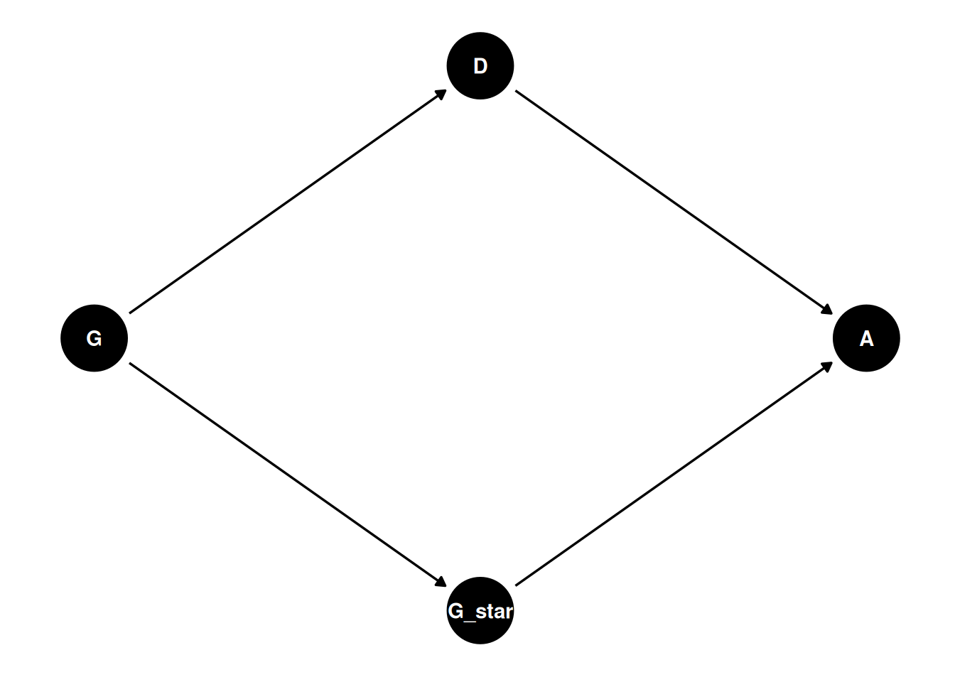
To calculate the causal effect of G*, we must average (marginalize) over the departments. (Note still assuming no confounds).
Simulate as if all applicants are women, then simulate as if all applicants are men. Then compute the contrasts.
Post stratification is reweighing estimates for target population. Eg. at a different university, the distributions would differ, and we could predict how the consequences of intervention differ
How long did an event take to happen? Time-to-event.
Cannot ignore censored cases, where event never happened.
Adoption rates of black and non-black cats
Events: adopted, or something else (death, escape, censored)
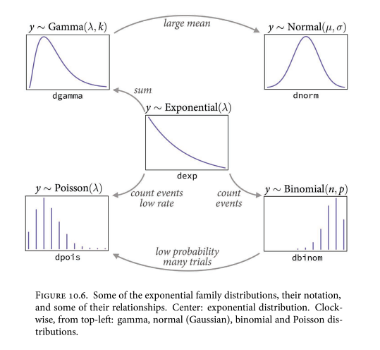
Outcome variables: days to event. Appropriate distributions are exponential and gamma. Exponential arises from a single part that needs to fail before the so-called machine dies, whereas the Gamma distribution requires multiple parts to fail.
For simplest situation, time to adoption, this represents it:
\(D_{i} \sim Exponential(\lambda_{i})\)
\(p(D_{i} | \lambda_{i}) = \lambda_{i} exp(-\lambda_{i} D_{i})\)
But what about the censored cats?
Event happened = cumulative distribution, probability of event happening up to time x
Event didn’t happen = complementary cumulative distribution, probability event hasn’t occurred up to time x
\(D_{i} = 1 \sim Exponential(\lambda_{i})\)
\(D_{i} = 0 \sim Exponential-CCDF(\lambda_{i})\) (not-yet-adoptions)
\(\lambda_{i} = 1 / \mu_{i}\)
\(log \mu_{i} = \alpha_{CID[i]}\)