Lecture 05 Notes

Author

Alec L. Robitaille

Published

February 13, 2023

The four elemental confounds

Correlation is common in nature, causation is sparse

Recall:

Estimand: goal
Estimator: recipe, instructions
Estimate: result, may not always match estimand due to eg. confounds

Confounds are features of the sample and how we use the sample that misleads us. Sources of confounds are diverse but there are four elemental confounds.

The fork

coords <- data.frame(
    name = c('X', 'Y', 'Z'),
    x =    c(1,    3,   2),
    y =    c(0,    0,   0)
)

dagify(
    X ~ Z,
    Y ~ Z,
  coords = coords
) |> ggdag(seed = 2, layout = 'auto') + theme_dag()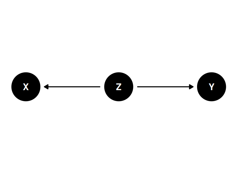

X and Y are associated (\(Y \not\!\perp\!\!\!\perp X\))
X and Y share common cause Z
Once stratified by Z, there will be no association (\(Y \perp\!\!\!\perp X | Z\))

\(\not\!\perp\!\!\!\perp\): not independent of

\(\perp\!\!\!\perp\): independent of

\(|\): conditional of

n <- 1e3
Z <- rbern(n, 0.5)
X <- rbern(n, (1-Z) * 0.1 + Z * 0.9)
Y <- rbern(n, (1-Z) * 0.1 + Z * 0.9)

table(X, Y)

   Y
X     0   1
  0 403  96
  1  97 404

cor(X, Y)

[1] 0.6140012

Example: marriage and divorce

Estimand: Why do regions of the USA with higher rates of marriage also have higher rates of divorce?

Age at marriage is also associated with divorce and marriage rates. Is the relationship between marriage rate and divorce rate solely a result of the fork, their shared relationship with age at marriage.

coords <- data.frame(
    name = c('M', 'D', 'A'),
    x =    c(1,    3,   2),
    y =    c(0,    0,   -1)
)

dagify(
    M ~ A,
    D ~ A + M,
  coords = coords
) |> ggdag(seed = 2, layout = 'auto') + theme_dag()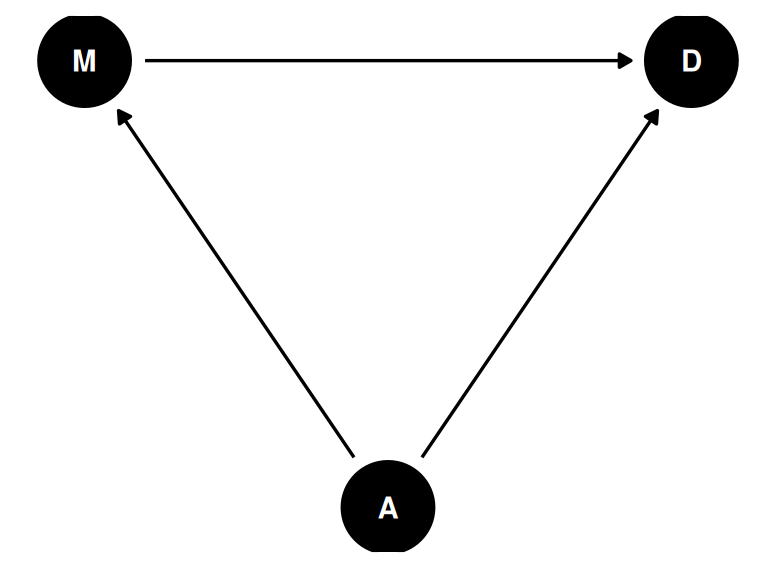

To estimate the causal effect of marriage rate, we need to stratify by age at marriage. Within each level of age at marriage, the part of the association between marriage rate and divorce rate that is caused by age at marriage is removed.

Stratifying by a continuous variable: every value of A produces a different relationship between D and M. We have a different expected relationship.

Statistical model

If we standardize (or rescale) the data, priors are easier to set for linear models. Standardize = subtract the mean (mean of 0) and divide by the standard deviation (sd of 1). “Since the outcome and the predictor are both standardized, the intercept should be very close to zero. The slope beta indicates that a change in one standard deviation in the predictor corresponds to a change in one standard deviation in the outcome” (Page 126).

Prior predictive simulation

n <- 100
ggplot() + 
    geom_abline(aes(intercept = rnorm(n, 0, 10), 
                                    slope = rnorm(n, 0, 10)),
                            alpha = 0.1, size = 2) + 
    labs(x = 'median age at marriage (standardized)', 
             y = 'divorce rate (standardized)') + 
    xlim(-2, 2) + 
    ylim(-2, 2)

Warning: Using `size` aesthetic for lines was deprecated in ggplot2 3.4.0.
ℹ Please use `linewidth` instead.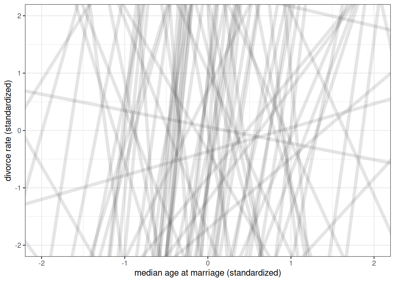

ggplot() + 
    geom_abline(aes(intercept = rnorm(n, 0, 0.2), 
                                    slope = rnorm(n, 0, 0.5)),
                            alpha = 0.1, size = 2) + 
    labs(x = 'median age at marriage (standardized)', 
             y = 'divorce rate (standardized)') + 
    xlim(-2, 2) + 
    ylim(-2, 2)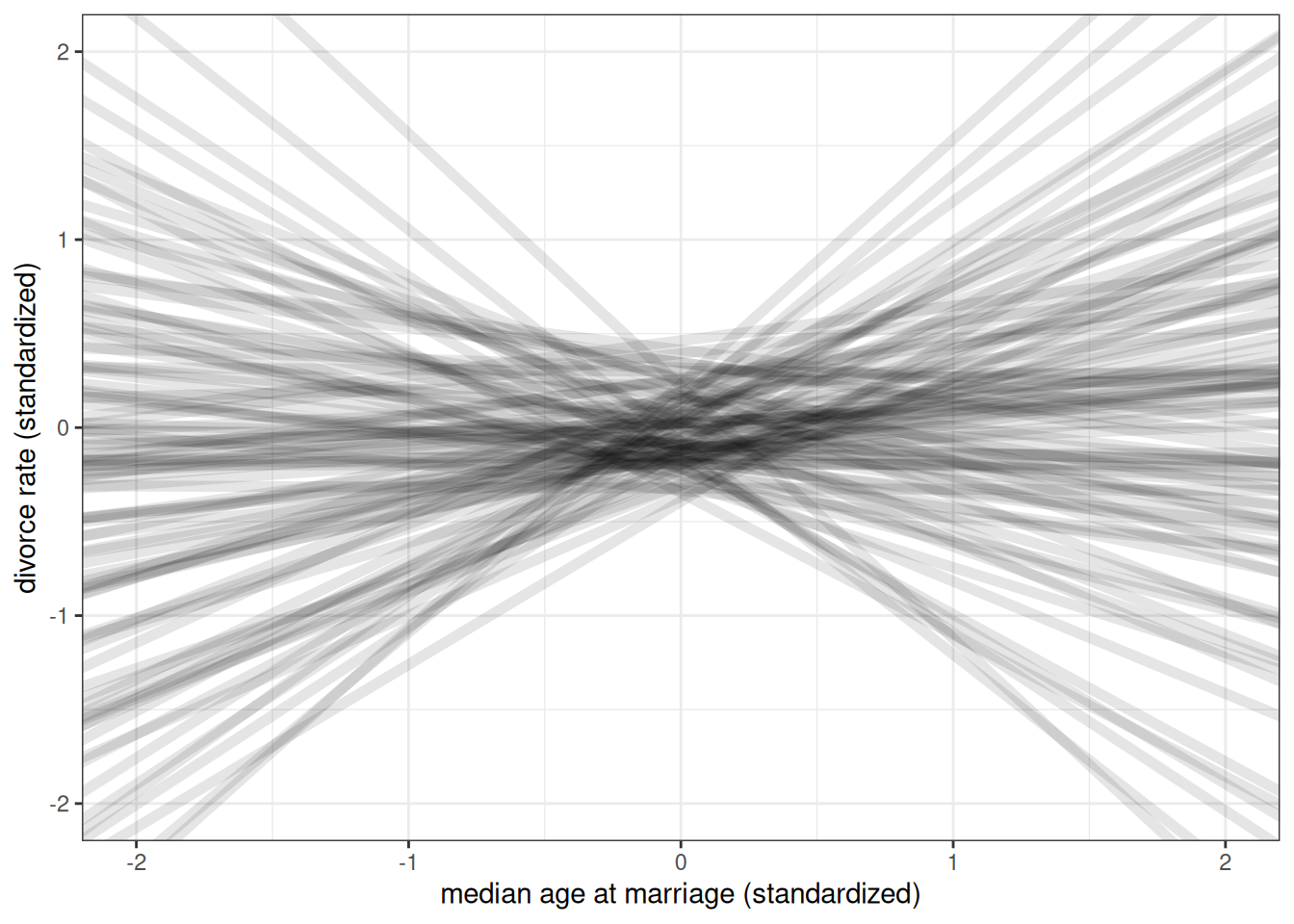

Analyze the data

The causal effect is not a function of one parameter, so reporting simply the mean estimated parameter is often insufficient especially when considering non-linear models or more complicated models.

Instead, simulate interventions.

\(p(D|do(M))\)

The distribution of D when we intervene (do) on M. This is different than

When we do(M), we remove all arrows into M. Using a common set of values for A, we set different values for M and see what difference it makes.

Generate common set of values for A
Set first value for M
Simulate for first value of M and common set of values for A
Set second value for M
Simulate for second value of M and common set of values for A
Compute the contrast

dagify(
    M ~ A,
    D ~ A + M,
  coords = coords
) |> ggdag(seed = 2, layout = 'auto') + theme_dag() +
    labs(title = 'no intervention') +
    dagify(
        D ~ A + M,
      coords = coords
) |> ggdag(seed = 2, layout = 'auto') + theme_dag() +
    labs(title = 'do(M)')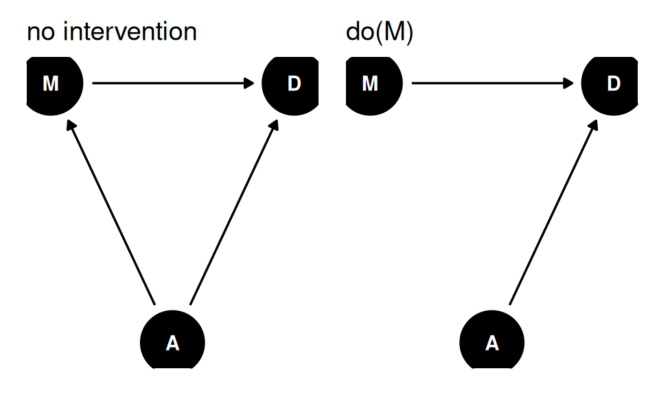

What about \(p(D|do(A))\)?

Total causal effect of A on D requires a new model, since M is a pipe between A and D.

The pipe

coords <- data.frame(
    name = c('X', 'Y', 'Z'),
    x =    c(1,    3,   2),
    y =    c(0,    0,   0)
)

dagify(
    Z ~ X,
    Y ~ Z,
  coords = coords
) |> ggdag(seed = 2, layout = 'auto') + theme_dag()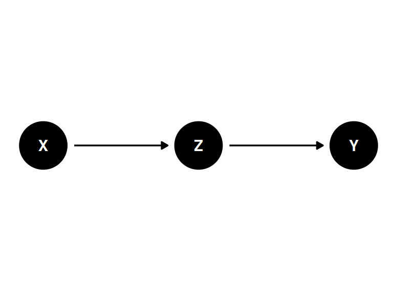

Z is a “mediator”

X and Y are associated (\(Y \not\!\perp\!\!\!\perp X\))
Influence of X on Y transmitted through Z
Once stratified by Z, there will be no association (\(Y \perp\!\!\!\perp X | Z\))

n <- 1e3
X <- rbern(n, 0.5)
Z <- rbern(n, (1-X) * 0.1 + X * 0.9)
Y <- rbern(n, (1-Z) * 0.1 + Z * 0.9)

table(X, Y)

   Y
X     0   1
  0 399 104
  1  89 408

cor(X, Y)

[1] 0.614332

table(X[Z == 0], Y[Z == 0])

cor(X[Z == 0], Y[Z == 0])

[1] 0.01934141

table(X[Z == 1], Y[Z == 1])

cor(X[Z == 1], Y[Z == 1])

[1] -0.04862018

Example: plant growth, anti-fungal

Estimand: causal effect of treatment (anti-fungal) on plant growth

coords <- data.frame(
    name = c('F', 'H1', 'H0', 'T'),
    x =    c(1,    2,   3, 0),
    y =    c(0,    1,   1, 1)
)

dagify(
    H1 ~ H0 + F + T,
    F ~ T,
  coords = coords
) |> ggdag(seed = 2, layout = 'auto') + theme_dag()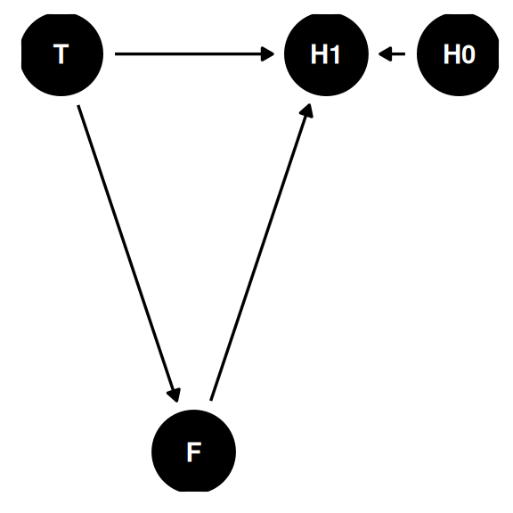

H0: height at time 0
H1: height at time 1
F: fungus
T: anti-fungal treatment

The path T -> F -> H1 is a pipe. Should we stratify by F? No. Total causal effect of treatment is blocked by the pipe through F.

This is post-treatment bias. Stratifying by a consequence of the treatment, misleading that treatment does or doesn’t work.

The collider

coords <- data.frame(
    name = c('X', 'Y', 'Z'),
    x =    c(1,    3,   2),
    y =    c(0,    0,   0)
)

dagify(
    Z ~ X + Y,
  coords = coords
) |> ggdag(seed = 2, layout = 'auto') + theme_dag()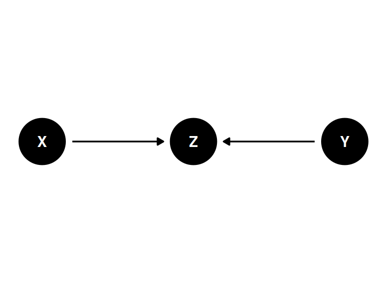

Z is a “collider”

X and Y are not associated (\(Y \perp\!\!\!\perp X\))
Z is caused by both X and Z
Once stratified by Z, X and Y are associated (\(Y \not\!\perp\!\!\!\perp X | Z\))

n <- 1e3
X <- rbern(n, 0.5)
Y <- rbern(n, 0.5)
Z <- rbern(n, ifelse(X + Y > 0, 0.9, 0.2))

table(X, Y)

   Y
X     0   1
  0 249 254
  1 250 247

cor(X, Y)

[1] -0.00798816

table(X[Z == 0], Y[Z == 0])

cor(X[Z == 0], Y[Z == 0])

[1] 0.3236048

table(X[Z == 1], Y[Z == 1])

cor(X[Z == 1], Y[Z == 1])

[1] -0.3202523

Example: grant applications

Each grant application scored on newsworthiness and trustworthiness

Grants are only awarded if sufficiently newsworthy or trustworthy. Few grants are high in both, therefore there is a negative association between newsworthiness and trustworthiness that arises from conditioning on awards. This is a post-selection sample, where the sample eg. awards or jobs have already selected for features.

Example: age and happiness

There are post-treatment colliders like the example above and there are colliders that are a result from the statistical processing, within the analysis.

Estimand: influence of age on happiness

Possible confound is marital status

coords <- data.frame(
    name = c('H', 'A', 'M'),
    x =    c(1,    3,   2),
    y =    c(0,    0,   0)
)

dagify(
    M ~ A + H,
  coords = coords
) |> ggdag(seed = 2, layout = 'auto') + theme_dag()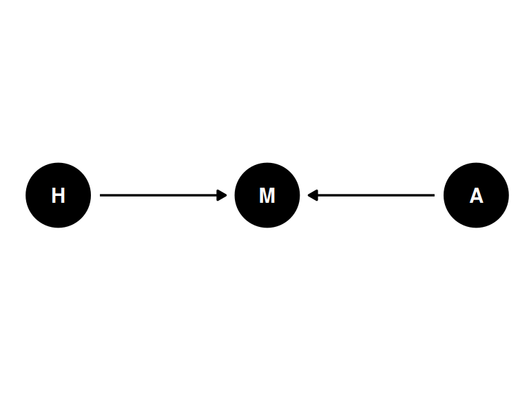

The descendant

coords <- data.frame(
    name = c('X', 'Y', 'Z', 'A'),
    x =    c(1,    3,   2, 2),
    y =    c(0,    0,   0, -1)
)

dagify(
    Z ~ X + Y,
    A ~ Z,
  coords = coords
) |> ggdag(seed = 2, layout = 'auto') + theme_dag()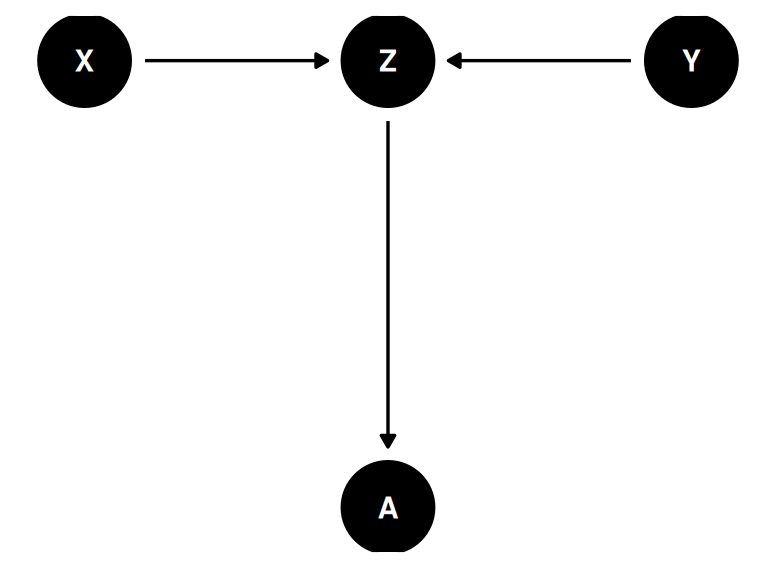

A is the descendant

Including A is like including Z

X and Y are causally associated through Z (\(Y \not\!\perp\!\!\!\perp X\))
A holds information about Z
Once stratified by A, X and Y are less associated (\(Y \perp\!\!\!\perp X | Z\))

n <- 1e3

X <- rbern(n, 0.5)
Z <- rbern(n, (1-X) * 0.1 + X * 0.9)
Y <- rbern(n, (1-Z) * 0.1 + Z * 0.9)
A <- rbern(n, (1-Z) * 0.1 + Z * 0.9)

table(X, Y)

   Y
X     0   1
  0 399 104
  1  89 408

cor(X, Y)

[1] 0.614332

table(X[A == 0], Y[A == 0])

cor(X[A == 0], Y[A == 0])

[1] 0.3855157

table(X[A == 1], Y[A == 1])

cor(X[A == 1], Y[A == 1])

[1] 0.33666

In this case, the correlation is reduced by about half.

Descendants are everywhere, because many measurements we have are