Varying intercepts on each district
\(C_{i} \sim Bernoulli(D_{i}, p_{i})\)
\(logit(p_{i}) = \alpha_{D[i]}\)
\(\alpha_{j} \sim Normal(\bar{\alpha}, \sigma)\)
\(\bar{\alpha} \sim Normal(0, 1)\)
\(\sigma \sim Exponential(1)\)
(Bernoulli distribution since contraception is 0/1 outcome)
Note the uneven sampling across districts, where because of partial pooling there is shrinkage in the clusters. More shrinkage in clusters with less observations eg. the districts with 2 and 13 observations, and less in clusters with more observations eg. the districts with 35 and 45 observations.
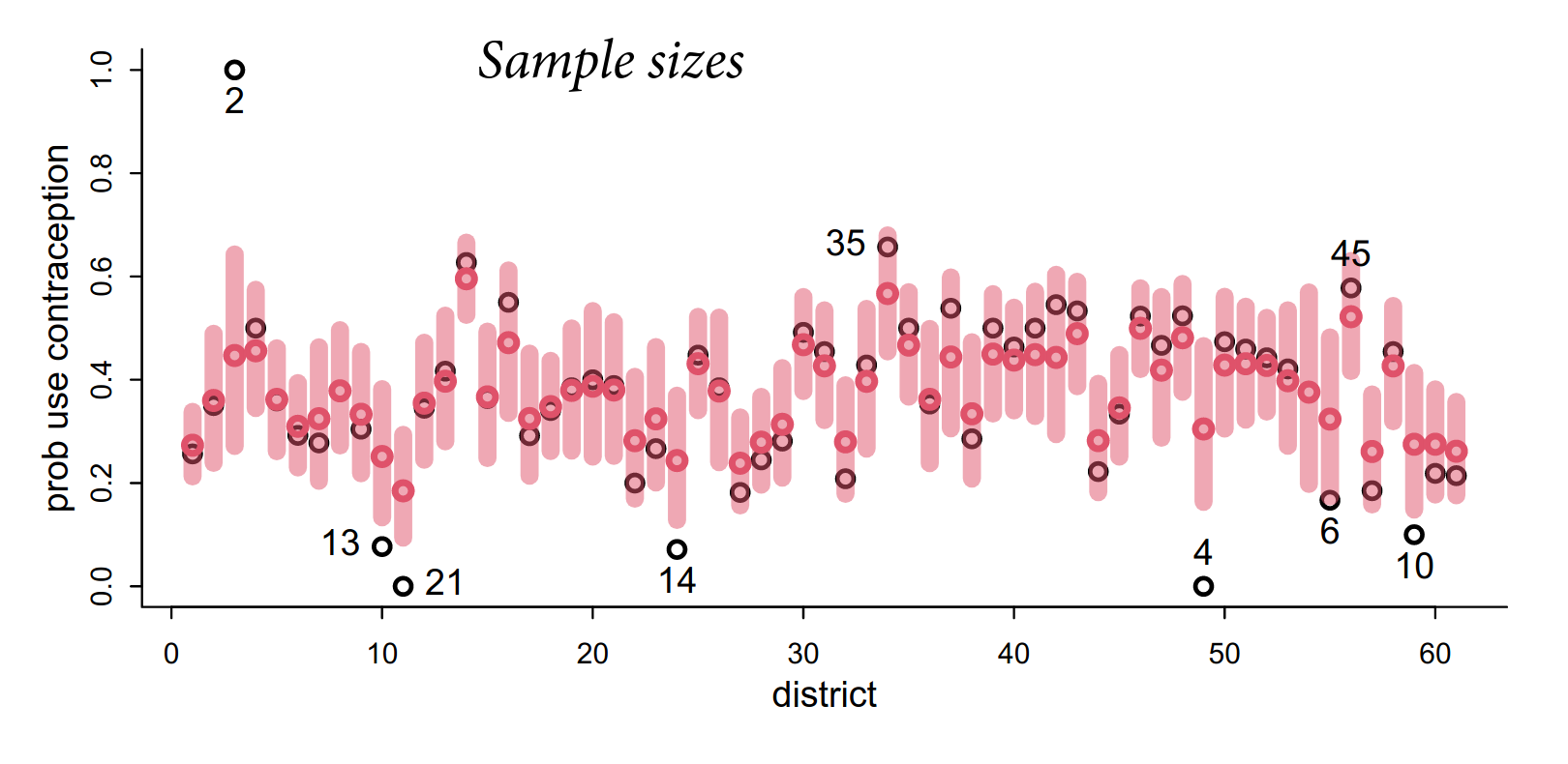
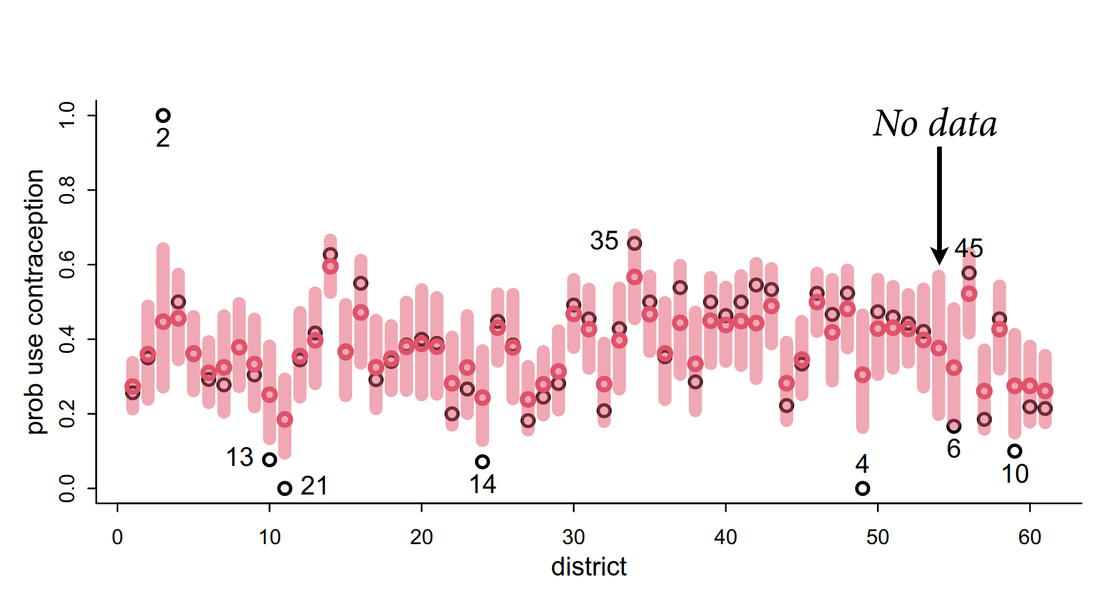
In addition, for one district there is no data. The minimum sample size is 0, because you have a prior. This is an informed prior because it is estimated from all the other districts, including the variation across all districts. This is in essence a prediction.
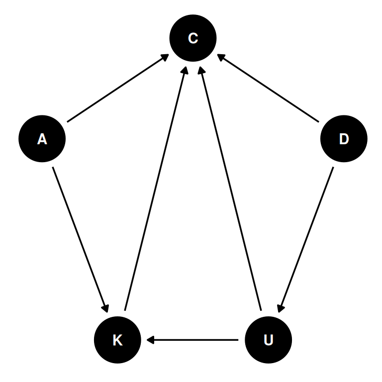
Varying intercepts on districts and slopes on urban
District features are potential group-level confounds. To estimate the total effect of urban (U), we need to stratify by district but not by kids (K) because the total effect of U passes through K.
\(C_{i} \sim Bernoulli(D_{i}, p_{i})\)
\(logit(p_{i}) = \alpha_{D[i]} + \beta_{D[i]}U_{i}\)
\(\alpha_{j} \sim Normal(\bar{\alpha}, \sigma)\)
\(\beta_{j} \sim Normal(\bar{\beta}, \tau)\)
\(\bar{\alpha}, \bar{\beta} \sim Normal(0, 1)\)
\(\sigma, \tau \sim Exponential(1)\)
Result: ~4/2000 transitions with a divergence. For 2000 samples, tau’s number of effective samples (n_eff) are quite low.
The problem is that there are priors that define the shape of other priors. They locate the priors, and are called “centered”. We can re-express the same thing using non-centered priors are that transformed to replace the nested priors with a Normal(0, 1) prior. These are mathematically equivalent but the non-centered model is much more efficient.
Z score is a standardized Gaussian deviation. Subtract by the mean and divide by the standard deviation. Easily reversible by adding the mean and multiplying by the standard deviation.
\(C_{i} \sim Bernoulli(D_{i}, p_{i})\)
\(logit(p_{i}) = \alpha_{D[i]} + \beta_{D[i]}U_{i}\)
\(\alpha_{j} = \bar{\alpha} + Z_{\alpha, j} * \sigma\)
\(\beta_{j} = \bar{\beta} + Z_{\beta, j} * \sigma\)
\(Z_{\alpha, j} \sim Normal(0, 1)\)
\(Z_{\beta, j} \sim Normal(0, 1)\)
\(\bar{\alpha}, \bar{\beta} \sim Normal(0, 1)\)
\(\sigma, \tau \sim Exponential(1)\)
Result: much more efficient sampling.
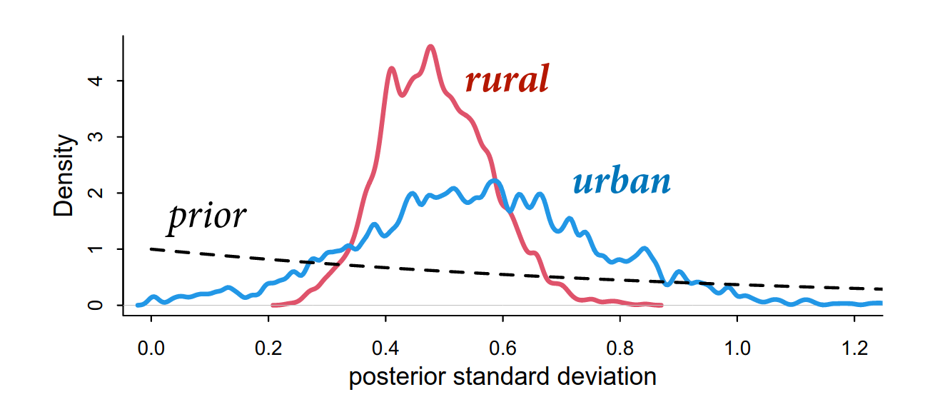
Sample size drops as you add more clusters and cut up the data.
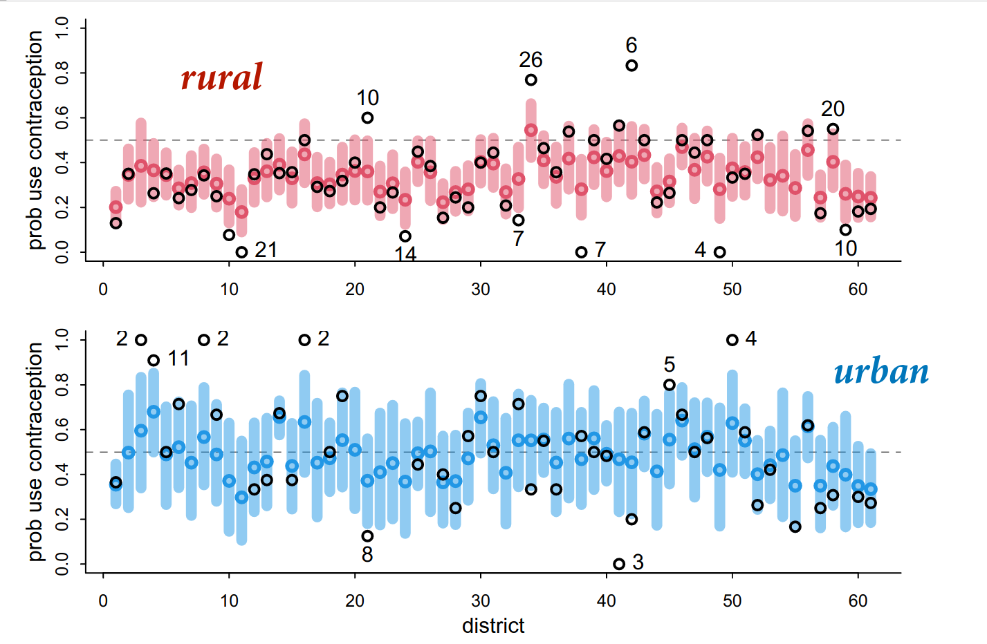 The urban estimates look more uncertain, possibly due to lower sample sizes in urban areas (there are less urban areas).