source('R/packages.R')Homework 03
Data
# Data
source('R/data_foxes.R')

# group : ID of group
# avgfood : Average available food in group's territory
# groupsize : Size of each group
# area : Area of group territory
# weight : Body weight of individual fox
DT <- data_foxes(scale = TRUE)
Scaling numeric variables: avgfood, groupsize, area, weightQuestion 1
The first two problems are based on the same data. The data in data(foxes) are 116 foxes from 30 different urban groups in England. These fox groups are like street gangs. Group size (groupsize) varies from 2 to 8 individuals. Each group maintains its own (almost exclusive) urban territory. Some ter- ritories are larger than others. The area variable encodes this information. Some territories also have more avgfood than others. And food influences the weight of each fox. Assume this following DAG. Use the backdoor criterion and estimate the total causal influence of A on F. What effect would increasing the area of a territory have on the amount of food inside it?
DAG
coords <- data.frame(
    name = c('A', 'F', 'G', 'W'),
    x =    c(2,    1,   3,    2),
    y =    c(3,    2,   2,    1)
)
dag <- dagify(
W ~ F + G,
F ~ A,
G ~ F,
coords = coords
)
dag |> ggdag(seed = 2) + theme_dag()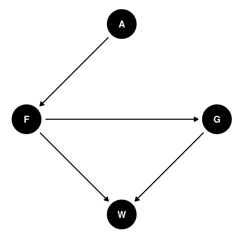
- A: area
- F: avgfood
- G: groupsize
- W: weight
Estimand
Total causal influence of area on average food. Consider how an intervention on area would influence average food.
adjustmentSets(dag, exposure = 'A', outcome = 'F', effect = 'total')Simulation
We don’t know much about this data, so to just get an idea of the units of the data, check the range of each column.
lapply(DT, range)$group
[1] 1 30
$avgfood
[1] 0.37 1.21
$groupsize
[1] 2 8
$area
[1] 1.09 5.07
$weight
[1] 1.92 7.55
$scale_avgfood
[1] -1.924829 2.310838
$scale_groupsize
[1] -1.524089 2.375785
$scale_area
[1] -2.239596 2.047562
$scale_weight
[1] -2.204059 2.550918But instead of peaking, let’s use the standardized versions and consider the potential effects on the scale of standard deviations.
tar_load(m_h03_q01_prior)
m_h03_q01_prior
Family: gaussian
Links: mu = identity; sigma = identity
Formula: scale_avgfood ~ scale_area
Data: foxes (Number of observations: 116)
Draws: 1 chains, each with iter = 2000; warmup = 1000; thin = 1;
total post-warmup draws = 1000
Population-Level Effects:
Estimate Est.Error l-95% CI u-95% CI Rhat Bulk_ESS Tail_ESS
Intercept -0.01 0.25 -0.49 0.51 1.00 711 604
scale_area -0.00 0.49 -1.03 0.94 1.00 839 655
Family Specific Parameters:
Estimate Est.Error l-95% CI u-95% CI Rhat Bulk_ESS Tail_ESS
sigma 1.00 0.97 0.04 3.53 1.00 810 447
Draws were sampled using sampling(NUTS). For each parameter, Bulk_ESS
and Tail_ESS are effective sample size measures, and Rhat is the potential
scale reduction factor on split chains (at convergence, Rhat = 1).# Formula
m_h03_q01_prior$formulascale_avgfood ~ scale_area # Priors
m_h03_q01_prior$prior prior class coef group resp dpar nlpar lb ub source
normal(0, 0.5) b user
normal(0, 0.5) b scale_area (vectorized)
normal(0, 0.25) Intercept user
exponential(1) sigma 0 user# Show draws from prior distributions
conditional_effects(m_h03_q01_prior, 'scale_area', prob = 0.89)
Model
tar_load(m_h03_q01)
m_h03_q01
Family: gaussian
Links: mu = identity; sigma = identity
Formula: scale_avgfood ~ scale_area
Data: foxes (Number of observations: 116)
Draws: 4 chains, each with iter = 2000; warmup = 1000; thin = 1;
total post-warmup draws = 4000
Population-Level Effects:
Estimate Est.Error l-95% CI u-95% CI Rhat Bulk_ESS Tail_ESS
Intercept -0.00 0.04 -0.09 0.09 1.00 3950 3115
scale_area 0.88 0.04 0.79 0.96 1.00 4246 3079
Family Specific Parameters:
Estimate Est.Error l-95% CI u-95% CI Rhat Bulk_ESS Tail_ESS
sigma 0.48 0.03 0.42 0.54 1.00 3741 2964
Draws were sampled using sampling(NUTS). For each parameter, Bulk_ESS
and Tail_ESS are effective sample size measures, and Rhat is the potential
scale reduction factor on split chains (at convergence, Rhat = 1).# Formula
m_h03_q01$formulascale_avgfood ~ scale_area # Priors
m_h03_q01$prior prior class coef group resp dpar nlpar lb ub source
normal(0, 0.5) b user
normal(0, 0.5) b scale_area (vectorized)
normal(0, 0.25) Intercept user
exponential(1) sigma 0 user# Parameter estimates
mcmc_areas(m_h03_q01, pars = c('b_Intercept', 'b_scale_area', 'sigma'))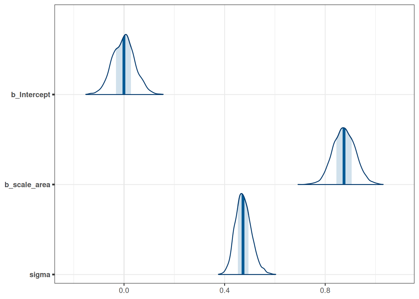
# Total causal influence of area on average food
conditional_effects(m_h03_q01, 'scale_area', prob = 0.89)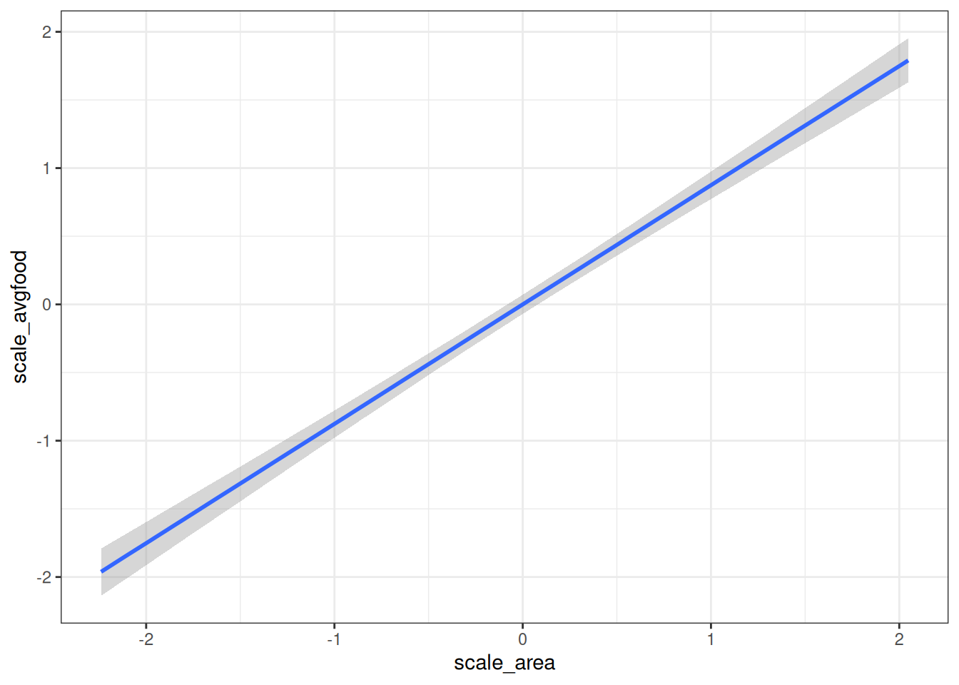
Question 2
Infer the total causal effect of adding food F to a territory on the weight W of foxes. Can you calculate the causal effect by simulating an intervention on food?
Estimand
Total causal influence of average food on weight. Consider how an intervention on average food would influence weight.
adjustmentSets(dag, exposure = 'F', outcome = 'W', effect = 'total')Simulation
tar_load(m_h03_q02_prior)

m_h03_q02_prior
Family: gaussian
Links: mu = identity; sigma = identity
Formula: scale_weight ~ scale_avgfood
Data: foxes (Number of observations: 116)
Draws: 1 chains, each with iter = 2000; warmup = 1000; thin = 1;
total post-warmup draws = 1000
Population-Level Effects:
Estimate Est.Error l-95% CI u-95% CI Rhat Bulk_ESS Tail_ESS
Intercept 0.00 0.26 -0.53 0.51 1.00 792 637
scale_avgfood 0.00 0.51 -0.95 1.01 1.00 609 576
Family Specific Parameters:
Estimate Est.Error l-95% CI u-95% CI Rhat Bulk_ESS Tail_ESS
sigma 1.04 1.05 0.02 3.88 1.00 584 367
Draws were sampled using sampling(NUTS). For each parameter, Bulk_ESS
and Tail_ESS are effective sample size measures, and Rhat is the potential
scale reduction factor on split chains (at convergence, Rhat = 1).# Formula
m_h03_q02_prior$formulascale_weight ~ scale_avgfood # Priors
m_h03_q02_prior$prior prior class coef group resp dpar nlpar lb ub
normal(0, 0.5) b
normal(0, 0.5) b scale_avgfood
normal(0, 0.25) Intercept
exponential(1) sigma 0
source
user
(vectorized)
user
user# Show draws from prior distributions
conditional_effects(m_h03_q02_prior, 'scale_avgfood', prob = 0.89)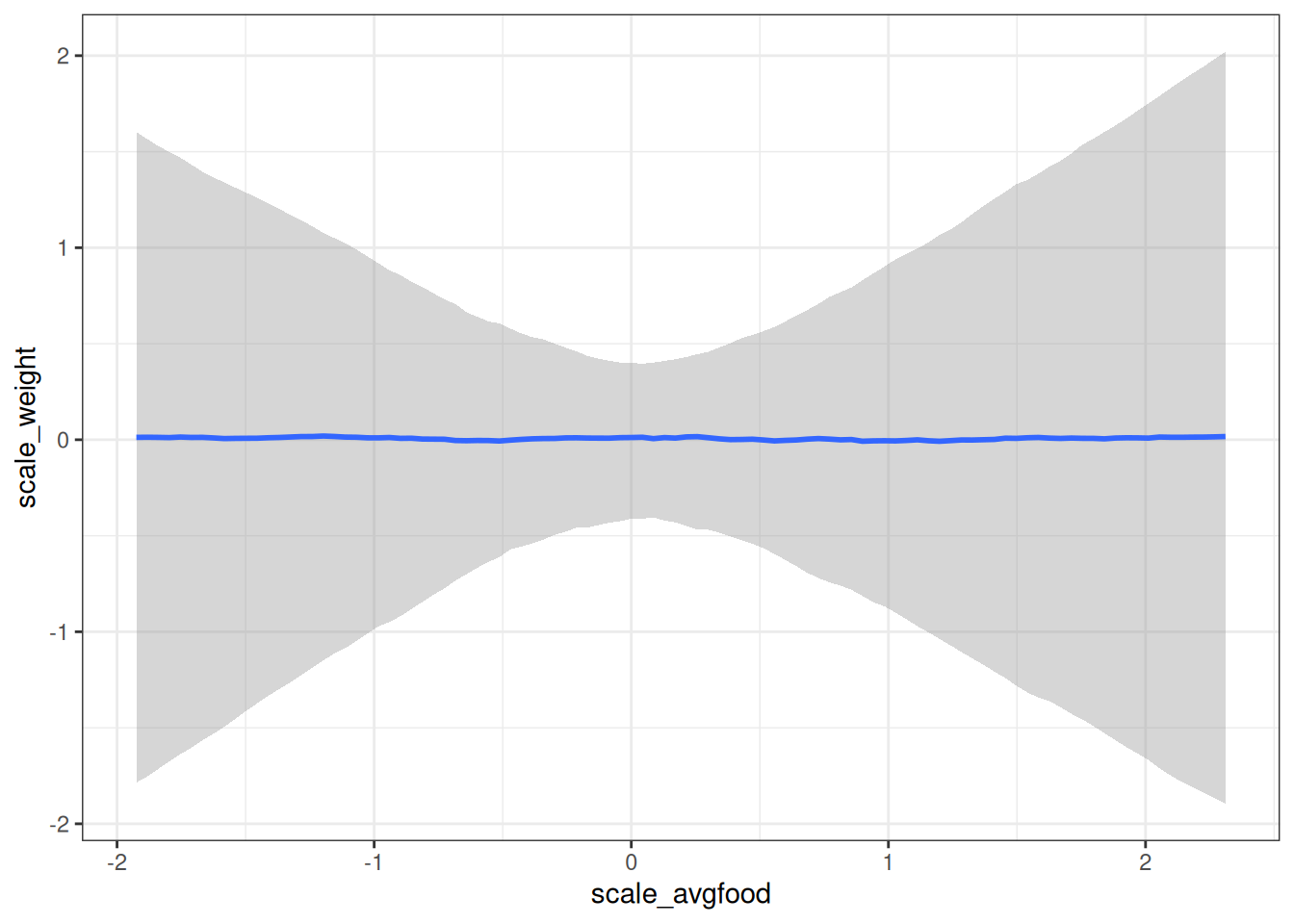
Model
tar_load(m_h03_q02)

m_h03_q02
Family: gaussian
Links: mu = identity; sigma = identity
Formula: scale_weight ~ scale_avgfood
Data: foxes (Number of observations: 116)
Draws: 4 chains, each with iter = 2000; warmup = 1000; thin = 1;
total post-warmup draws = 4000
Population-Level Effects:
Estimate Est.Error l-95% CI u-95% CI Rhat Bulk_ESS Tail_ESS
Intercept -0.00 0.09 -0.18 0.17 1.00 3538 2939
scale_avgfood -0.02 0.09 -0.21 0.17 1.00 3305 2894
Family Specific Parameters:
Estimate Est.Error l-95% CI u-95% CI Rhat Bulk_ESS Tail_ESS
sigma 1.01 0.07 0.89 1.16 1.00 3917 2888
Draws were sampled using sampling(NUTS). For each parameter, Bulk_ESS
and Tail_ESS are effective sample size measures, and Rhat is the potential
scale reduction factor on split chains (at convergence, Rhat = 1).# Formula
m_h03_q02$formulascale_weight ~ scale_avgfood # Priors
m_h03_q02$prior prior class coef group resp dpar nlpar lb ub
normal(0, 0.5) b
normal(0, 0.5) b scale_avgfood
normal(0, 0.25) Intercept
exponential(1) sigma 0
source
user
(vectorized)
user
user# Parameter estimates
mcmc_areas(m_h03_q02, pars = c('b_Intercept', 'b_scale_avgfood', 'sigma'))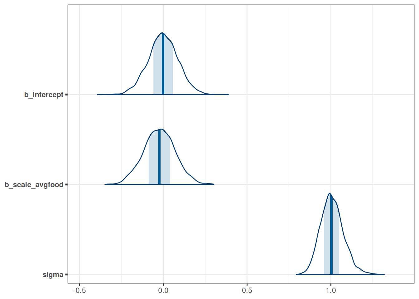
# Total causal influence of average food on weight
conditional_effects(m_h03_q02, 'scale_avgfood', prob = 0.89)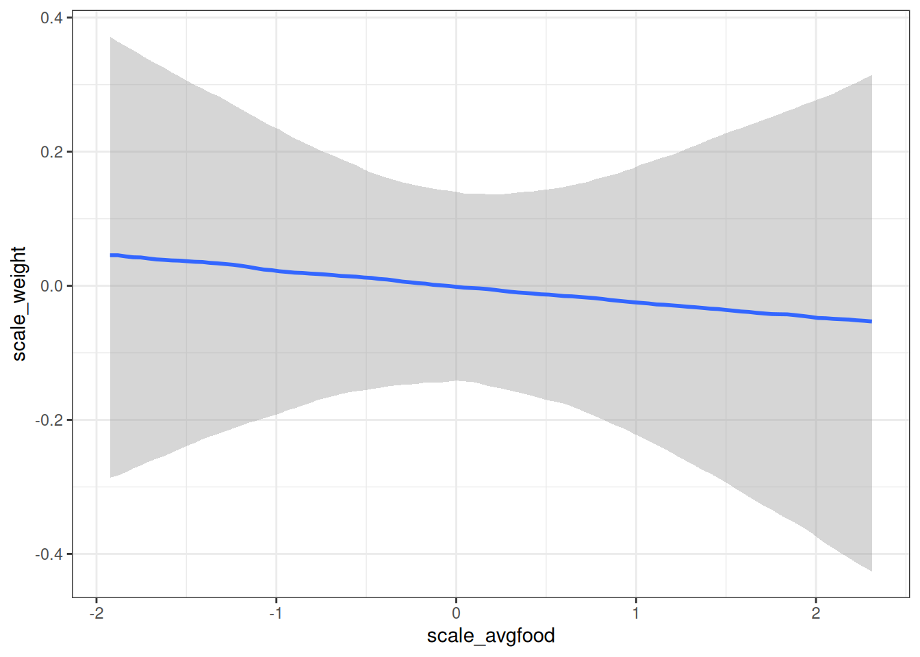
Question 3
Infer the direct causal effect of adding food F to a territory on the weight W of foxes. In light of your estimates from this problem and the previous one, what do you think is going on with these foxes?
Estimand
Direct causal influence of average food on weight. Consider how an intervention on average food would influence weight.
adjustmentSets(dag, exposure = 'F', outcome = 'W', effect = 'direct'){ G }Simulation
tar_load(m_h03_q03_prior)

# Formula
m_h03_q03_prior$formula
scale_weight ~ scale_avgfood + scale_groupsize # Priors
m_h03_q03_prior$prior prior class coef group resp dpar nlpar lb ub
normal(0, 0.5) b
normal(0, 0.5) b scale_avgfood
normal(0, 0.5) b scale_groupsize
normal(0, 0.25) Intercept
exponential(1) sigma 0
source
user
(vectorized)
(vectorized)
user
user# Show draws from prior distributions
conditional_effects(m_h03_q03_prior, 'scale_avgfood', prob = 0.89)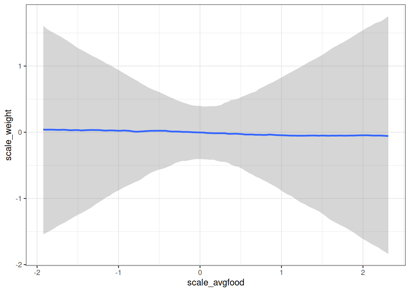
Model
tar_load(m_h03_q03)

m_h03_q03
Family: gaussian
Links: mu = identity; sigma = identity
Formula: scale_weight ~ scale_avgfood + scale_groupsize
Data: foxes (Number of observations: 116)
Draws: 4 chains, each with iter = 2000; warmup = 1000; thin = 1;
total post-warmup draws = 4000
Population-Level Effects:
Estimate Est.Error l-95% CI u-95% CI Rhat Bulk_ESS Tail_ESS
Intercept -0.00 0.08 -0.16 0.16 1.00 2788 2620
scale_avgfood 0.47 0.18 0.10 0.83 1.00 1990 1966
scale_groupsize -0.57 0.18 -0.92 -0.19 1.00 1909 1810
Family Specific Parameters:
Estimate Est.Error l-95% CI u-95% CI Rhat Bulk_ESS Tail_ESS
sigma 0.96 0.06 0.84 1.09 1.00 2986 2464
Draws were sampled using sampling(NUTS). For each parameter, Bulk_ESS
and Tail_ESS are effective sample size measures, and Rhat is the potential
scale reduction factor on split chains (at convergence, Rhat = 1).# Formula
m_h03_q03$formulascale_weight ~ scale_avgfood + scale_groupsize # Priors
m_h03_q03$prior prior class coef group resp dpar nlpar lb ub
normal(0, 0.5) b
normal(0, 0.5) b scale_avgfood
normal(0, 0.5) b scale_groupsize
normal(0, 0.25) Intercept
exponential(1) sigma 0
source
user
(vectorized)
(vectorized)
user
user# Parameter estimates
mcmc_areas(m_h03_q03, pars = c('b_Intercept', 'b_scale_avgfood', 'sigma'))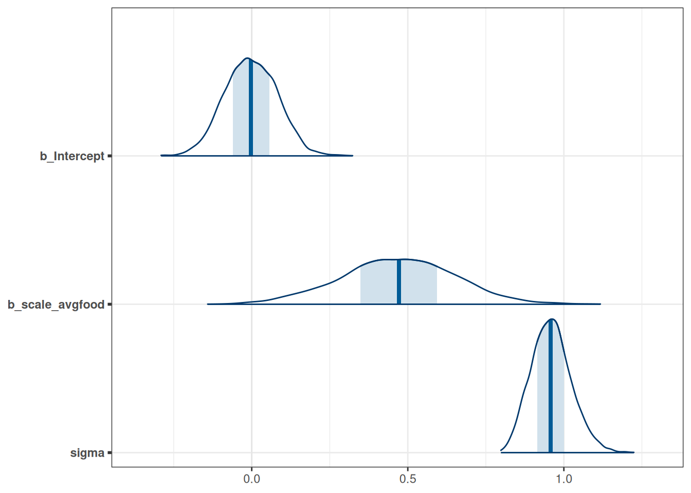
# Direct causal influence of average food on weight
conditional_effects(m_h03_q03, 'scale_avgfood', prob = 0.89)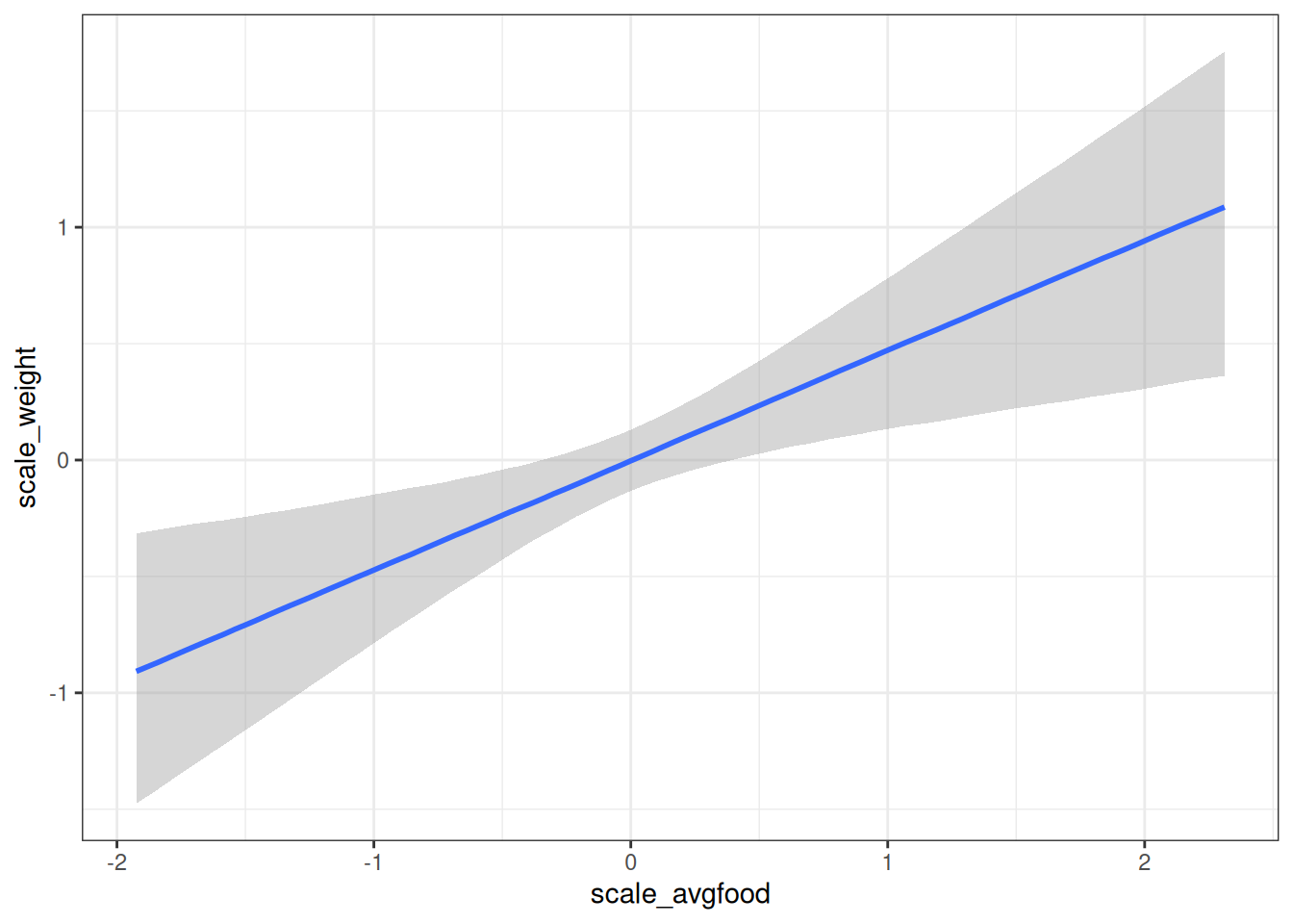
Closing the backdoor path and estimating the direct effect of average food on weight now shows a positive relationship between average food and fox weight.
conditional_effects(m_h03_q03, 'scale_groupsize', prob = 0.89)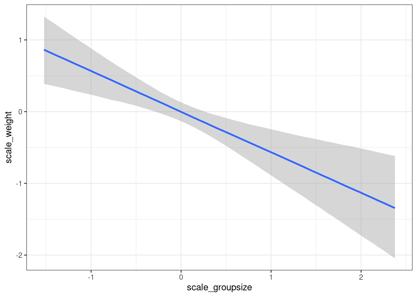
#| warning: false
tar_load(m_h03_q03_groupsize_food)

m_h03_q03_groupsize_food
Family: gaussian
Links: mu = identity; sigma = identity
Formula: scale_groupsize ~ scale_avgfood
Data: foxes (Number of observations: 116)
Draws: 4 chains, each with iter = 2000; warmup = 1000; thin = 1;
total post-warmup draws = 4000
Population-Level Effects:
Estimate Est.Error l-95% CI u-95% CI Rhat Bulk_ESS Tail_ESS
Intercept 0.00 0.04 -0.08 0.08 1.00 3844 3147
scale_avgfood 0.89 0.04 0.81 0.98 1.00 3533 2732
Family Specific Parameters:
Estimate Est.Error l-95% CI u-95% CI Rhat Bulk_ESS Tail_ESS
sigma 0.44 0.03 0.39 0.50 1.00 3809 2817
Draws were sampled using sampling(NUTS). For each parameter, Bulk_ESS
and Tail_ESS are effective sample size measures, and Rhat is the potential
scale reduction factor on split chains (at convergence, Rhat = 1).# Formula
m_h03_q03_groupsize_food$formulascale_groupsize ~ scale_avgfood # Priors
m_h03_q03_groupsize_food$prior prior class coef group resp dpar nlpar lb ub
normal(0, 0.5) b
normal(0, 0.5) b scale_avgfood
normal(0, 0.25) Intercept
exponential(1) sigma 0
source
user
(vectorized)
user
user# Direct causal influence of average food on group size
conditional_effects(m_h03_q03_groupsize_food, 'scale_avgfood', prob = 0.89)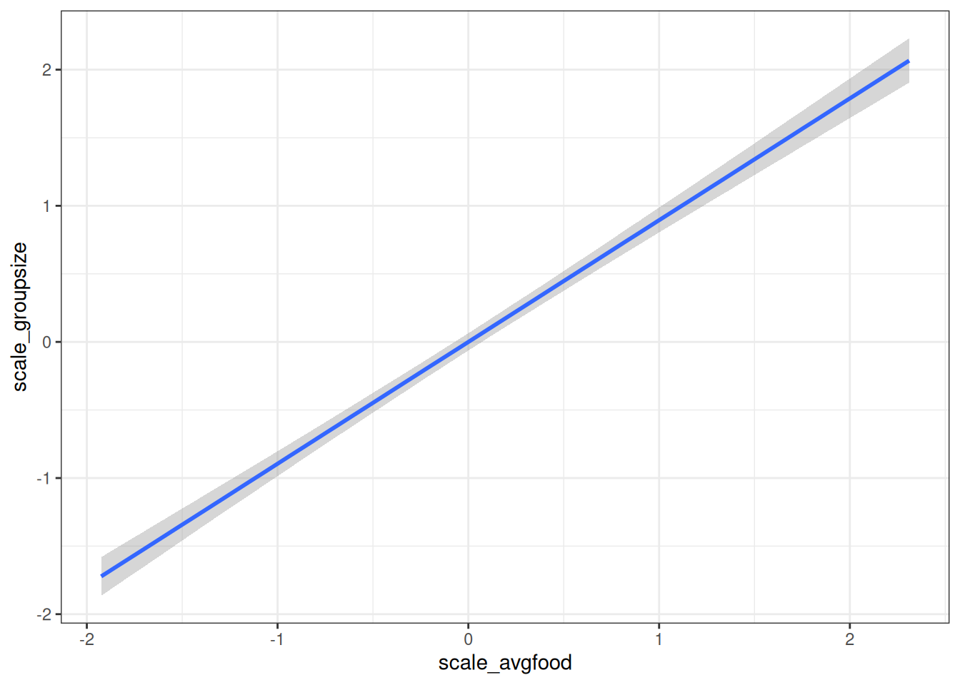
As average food in a territory increases, the group size increases.
Question 4 (bonus)
Suppose there is an unobserved confound that influences F and G. Assuming the DAG above is correct, again estimate both the total and direct causal effects of F on W. What impact does the unobserved confound have?
coords <- data.frame(
    name = c('A', 'F', 'G', 'W', 'U'),
    x =    c(1,    1,   2,    1.5,   2),
    y =    c(3,    2,   2,    1,   3)
)
dag <- dagify(
W ~ F + G,
F ~ A + U,
G ~ F + U,
coords = coords,
latent = 'U'
)
dag |> ggdag(seed = 2) + theme_dag()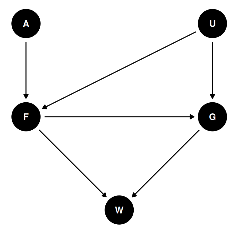
Estimand
Total and direct causal effects of F on W.
adjustmentSets(dag, exposure = 'F', outcome = 'W', effect = 'total')adjustmentSets(dag, exposure = 'F', outcome = 'W', effect = 'direct'){ G }In estimating the total causal effect of average food on weight, the unobserved confound U opens a backdoor on average food through group size. If group size is included, the direct effect will be estimated and not the total effect.