Lecture 12 Notes

Multilevel models

Repeat observations within groups can be modeled using categorical variables eg. a vector of alphas for each individual. Categorical variables have anterograde amnesia, when estimating eg. the beta for a new individual, this estimate does not contribute anything to the next individual.

Multilevel models instead, have two kinds of models

1. Model observations (eg. responses) of groups/individuals
2. Model population of groups/individuals (clusters)

The population model creates a kind of memory. Advantages of multilevel model include:

• more efficient estimation
• resists overfitting

The order that we estimate clusters does not matter, because we update the population level model with every cluster estimate and that population level model contributes to all clusters’ estimates. The information gathered from each cluster is pooled.

Regularization

Types of pooling

• Complete pooling: all clusters are the same. This results in underfitting.
• No pooling: all clusters are unrelated. This results in overfitting.
• Partial pooling: adaptive compromise. There is shrinkage towards the global mean.

Regularization with multilevel models is partial pooling, an adaptive compromise.

Example: cafes

Grey distribution is the priors Red distribution is the posterior Blue distribution is the population

Example: reedfrogs

• 48 tanks (T) of reedfrogs
• treatments: density (D), size (G), predation (P)
• outcome: survival (S)

coords <- data.frame(
    name = c('D', 'G', 'P', 'T', 'S'),
    x =    c(1,    2,   3,   1,    2),
    y =    c(0,    0,   0,   1,  1)
)

dagify(
    S ~ D + G + P + T,
  coords = coords
) |> ggdag(seed = 2, layout = 'auto') + theme_dag()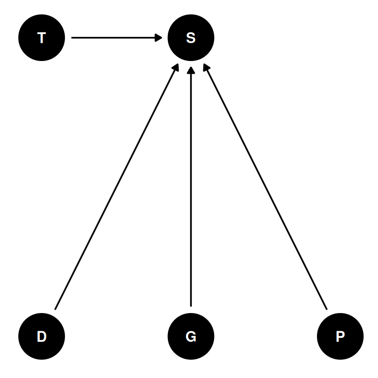

\(S_{i} \sim Binomial(D_{i}, p_{i})\)

\(logit(p_{i}) = \alpha_{T[i]}\)

\(\alpha_{j} \sim Normal(\bar{\alpha}, \sigma)\)

\(\bar{\alpha} \sim Normal(0, 1.5)\)

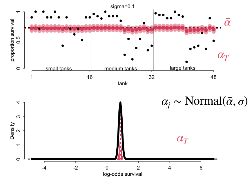
Sigma

\(\alpha_{j} \sim Normal(\bar{\alpha}, 0.1)\)

At sigma = 0.1, we tell the model that the tanks are all very similar and the result is estimates for each tank that are all close to the average.

\(\alpha_{j} \sim Normal(\bar{\alpha}, 5)\)

At sigma = 5, we tell the model that the tanks vary a lot and the prior does not create any constraints. This is equivalent to a categorical variable with amnesia with estimates very close to their values with in essence no pooling across tanks.

There is an optimal sigma for learning between total pooling/underfitting and no pooling/overfitting. We can find the optimal sigma using cross validation and comparing the PSIS values of each model. Note this is different than defining a prior using the model fit to the sample data because we are evaluating how the model fits to out of sample data (cross validation).

\(\alpha_{j} \sim Normal(\bar{\alpha}, 1.79)\)

At the optimal sigma determined for this data, the estimate is not exactly at the value and we see shrinkage across the tanks towards the global mean.

Alternatively, we can estimate as a parameter in the model.

\(S_{i} \sim Binomial(D_{i}, p_{i})\)

\(logit(p_{i}) = \alpha_{T[i]}\)

\(\alpha_{j} \sim Normal(\bar{\alpha}, \sigma)\)

\(\bar{\alpha} \sim Normal(0, 1.5)\)

\(\sigma \sim Exponential(1)\)

Estimates

Note that estimates for smaller tanks (with less frogs/observations) have smaller evidence and result in more conservative estimates (closer) to the global mean. Alternatively, larger tanks with more observations are less conservative.

Predators

Add a beta for predators, estimate a reduction in tank level survival (obviously). But the interesting thing is that the predictions between the model with and without predators is extremely similar. The difference is, however, in the sigma values where the model with predators has an estimate sigma around half that of the model without predators. The predator variable has explained approximately half of the variation on the log odds scale of the tanks.

The sigma is not the variation among the units, it’s the variation among the parameters net all the other effects in the model.

Varying effects

Recommended default is to use partial pooling if there are >1 clusters

Superstitions:

1. Units must be sampled at random
2. Number of units must be large
3. Assumes Gaussian variation

Practical difficulties

1. How to use more than one cluster type at the same time
2. How to sample efficiently
3. Slopes and confounds

Bonus: random confounds

Random confounds, when unobserved group features influence individually-varying causes. Group-level variables can have direct and indirect influences. Unmeasured features of the group can affect the response directly and indirectly through the traits of individuals.

Related terminology..

• group-level confounding
• endogeneity
• correlated errors
• econometrics

Options:

1. Fixed effects model. Inefficient but soak up group-level confounding. Cannot identify group-level effects.
2. Multilevel model. Better estimates for group-level variables but worse estimates for individual-level effects.
3. Mundlak machine. Estimate a different average rate for each group but not efficient and doesn’t respect the uncertainty in X-bar.

Or use a latent measurement error model.

Example: reedfrogs

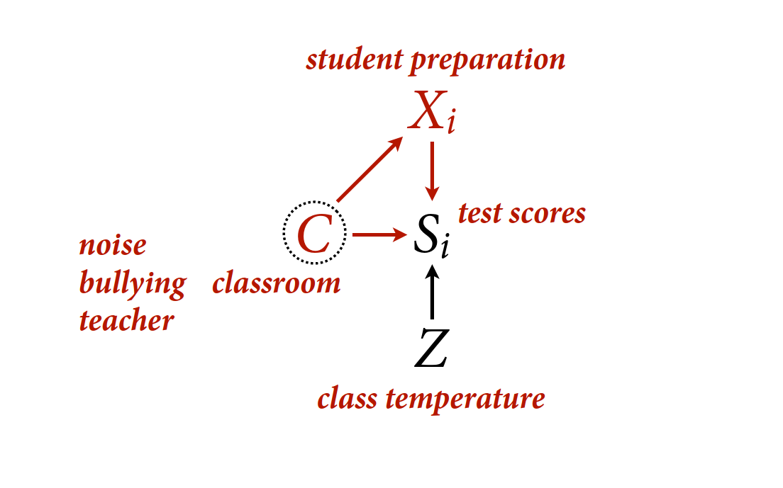
Estimand: \(p(S|do(X))\), the distribution of survival intervening on X.

The problem: there is a backdoor path through G

• Z group level trait
• X individual level trait

coords <- data.frame(
    name = c('G', 'S', 'X', 'Z'),
    x =    c(1,    2,    2,   2),
    y =    c(0,    0,    2,  -1)
)

dagify(
    S ~ G + X + Z,
    X ~ G,
  coords = coords
) |> ggdag(seed = 2, layout = 'auto') + theme_dag()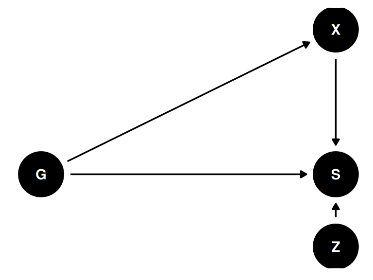

Example: classrooms