Homework 01

Question 1

Suppose the globe tossing data (Lecture 2, Chapter 2) had turned out to be 4 water and 11 land. Construct the posterior distribution.

source('R/packages.R')

qs 0.25.7

Loading required package: usethis

Attaching package: 'ggdag'

The following object is masked from 'package:stats':

    filter

This is cmdstanr version 0.7.1

- CmdStanR documentation and vignettes: mc-stan.org/cmdstanr

- CmdStan path: /home/alecr/.cmdstan/cmdstan-2.33.1

- CmdStan version: 2.33.1

A newer version of CmdStan is available. See ?install_cmdstan() to install it.
To disable this check set option or environment variable CMDSTANR_NO_VER_CHECK=TRUE.

Loading required package: posterior

This is posterior version 1.5.0

Attaching package: 'posterior'

The following objects are masked from 'package:stats':

    mad, sd, var

The following objects are masked from 'package:base':

    %in%, match

Loading required package: parallel

rethinking (Version 2.40)

Attaching package: 'rethinking'

The following object is masked from 'package:stats':

    rstudent

Loading required package: Rcpp

Loading 'brms' package (version 2.20.4). Useful instructions
can be found by typing help('brms'). A more detailed introduction
to the package is available through vignette('brms_overview').

Attaching package: 'brms'

The following objects are masked from 'package:rethinking':

    LOO, stancode, WAIC

The following objects are masked from 'package:ggdist':

    dstudent_t, pstudent_t, qstudent_t, rstudent_t

The following object is masked from 'package:stats':

    ar

Attaching package: 'tidybayes'

The following objects are masked from 'package:brms':

    dstudent_t, pstudent_t, qstudent_t, rstudent_t

This is bayesplot version 1.10.0

- Online documentation and vignettes at mc-stan.org/bayesplot

- bayesplot theme set to bayesplot::theme_default()

   * Does _not_ affect other ggplot2 plots

   * See ?bayesplot_theme_set for details on theme setting

Attaching package: 'bayesplot'

The following object is masked from 'package:brms':

    rhat

The following object is masked from 'package:posterior':

    rhat

Attaching package: 'emmeans'

The following object is masked from 'package:devtools':

    test

Attaching package: 'mice'

The following object is masked from 'package:stats':

    filter

The following objects are masked from 'package:base':

    cbind, rbind

Attaching package: 'janitor'

The following objects are masked from 'package:stats':

    chisq.test, fisher.test

source('R/compute_posterior_globe.R')

n_water <- 4
n_land <- 11
x <- c(rep('W', n_water), rep('L', n_land))
n_possibilities <- 5
posterior <- compute_posterior_globe(x, n_possibilities = n_possibilities)

kable(posterior, digits = 4)

W	L	possibility	ways	post
4	11	0.00	0	0.0000
4	11	0.25	177147	0.8436
4	11	0.50	32768	0.1560
4	11	0.75	81	0.0004
4	11	1.00	0	0.0000

# Using a finer grid with more potential possibilities
n_possibilities <- 100
posterior <- compute_posterior_globe(x, n_possibilities = n_possibilities)

Question 2

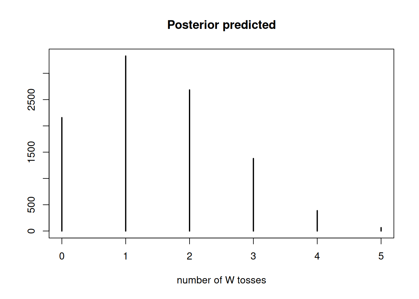
Using the posterior distribution from 1, compute the posterior predictive distribution for the next 5 tosses of the same globe. I recommend you use the sampling method.

possibilities <- seq(0, 1, length.out = n_possibilities)
size <- 1e4
n_tosses <- 5


# == Sampling approach from posterior
# Sample with probability posterior distribution calculated in Question 1
# using the grid of possibilities (sequence of numbers between 0 and 1)
posterior_samples <- sample(
    possibilities,
    size = size,
    prob = posterior$post,
    replace = TRUE
)

# Using the posterior predicted proportion of water, simulate 5 tosses for each
posterior_predict <- rbinom(size, size = n_tosses, p = posterior_samples)

# Plot number of W tosses 
plot(table(posterior_predict), xlab = 'number of W tosses', ylab = '', 
         main = 'Posterior predicted')

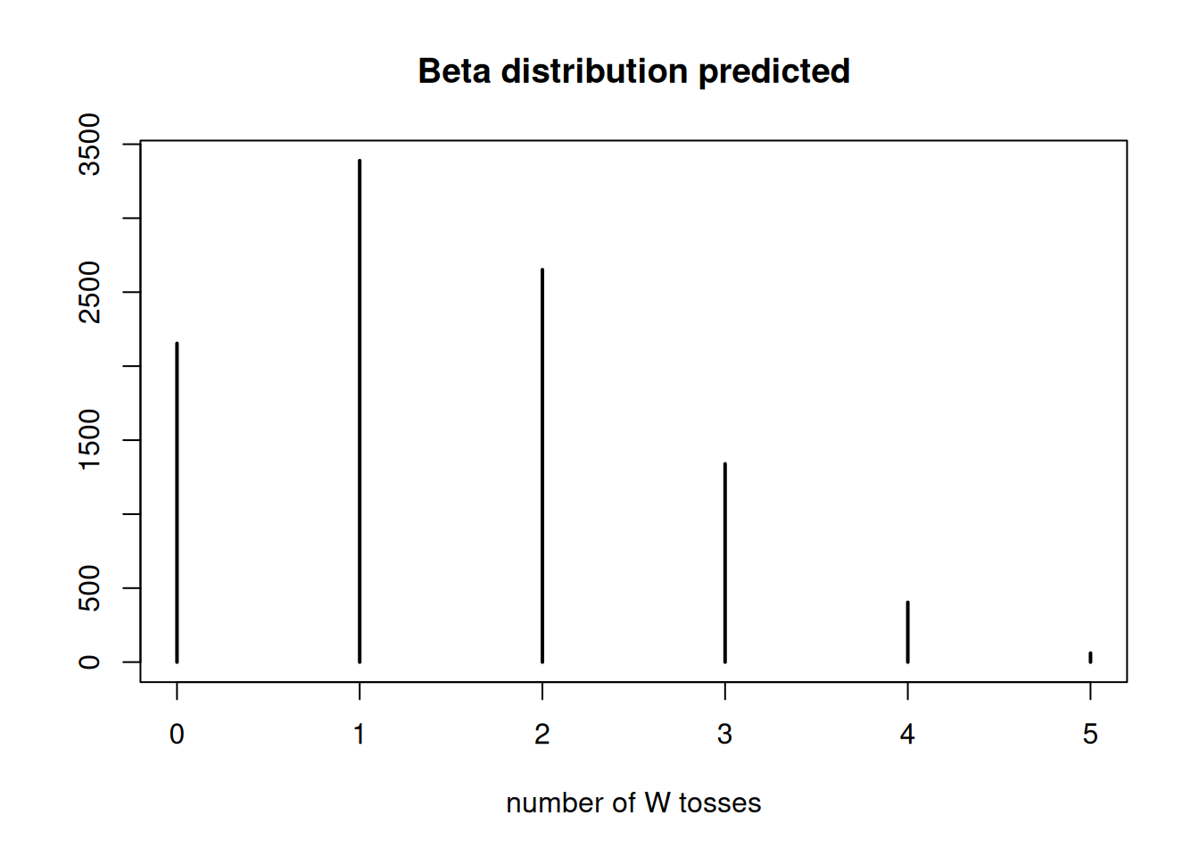
# === Sampling approach from representative Beta distribution
beta_samples <- rbeta(
    size,
    n_water + 1,
    n_land + 1
)

# Using the beta distribution predicted proportion of water, simulate 5 tosses for each
beta_predict <- rbinom(size, size = n_tosses, p = beta_samples)

# Plot number of W tosses 
plot(table(beta_predict), xlab = 'number of W tosses', ylab = '', 
         main = 'Beta distribution predicted')

Question 3

Use the posterior predictive distribution from 2 to calculate the probability of 3 or more water samples in the next 5 tosses.

# Predicted probability of 3 or more water samples in the next 5 tosses
#  given posterior predictive distribution
table(posterior_predict >= 3) / size

FALSE  TRUE 
0.817 0.183 

# and beta distribution prediction
table(beta_predict >= 3) / size

 FALSE   TRUE 
0.8195 0.1805 

Question 4 (optional)

This problem is an optional challenge for people who are taking the course for a second or third time. Suppose you observe W = 5 water points, but you forgot to write down how many times the globe was tossed, so you don’t know the number of land points L. Assume that p = 0.7 and compute the posterior distribution of the number of tosses N. Hint: Use the binomial distribution.

p <- 0.7
n_water <- 5

n_samples <- seq(5, 15)

d <- vapply(n_samples, dbinom, x = n_water, prob = p, FUN.VALUE = 42)

kable(data.table(
    n_samples = n_samples,
    post = d
))

n_samples	post
5	0.1680700
6	0.3025260
7	0.3176523
8	0.2541218
9	0.1715322
10	0.1029193
11	0.0566056
12	0.0291115
13	0.0141918
14	0.0066229
15	0.0029803