Lecture 14 Notes

Author

Alec L. Robitaille

Published

February 17, 2023

Correlated features

One prior distribution for each cluster

  1. One feature: one-dimensional distribution
  2. Two features: two-dimensional distribution
  3. N features: N-dimensional distribution

\([\alpha_{j}, \beta_{j}] \sim MVNormal([\bar{\alpha}, \bar{\beta}], R, [\sigma, \tau])\)

  • \([\alpha_{j}, \beta_{j}]\): features for district j
  • \(MVNormal\)
    • \([\bar{\alpha}, \bar{\beta}]\): feature means
    • \(R\): correlation matrix
    • \([\sigma, \tau])\): standard deviations

\(R \sim LKJCorr(4)\)

The LKJ prior is a prior distribution for correlations.

See here for plotting LKJCorr distributions.

Example: Bangladesh fertility survey

Outcome: contraceptive use

Variables: age, living children, urban/rural, districts

coords <- data.frame(
    name = c('A', 'C', 'D', 'K', 'U'),
    x =    c(1,    2,    3,   1.5, 2.5),
    y =    c(0,    0.5,    0,  -1, -1)
)
dagify(
    C ~ A + K + D + U,
    K ~ A + U,
    U ~ D,
  coords = coords
) |> ggdag(seed = 2, layout = 'auto') + theme_dag()

From the previous lecture, the varying intercepts for district and slopes for urban.

\(C_{i} \sim Bernoulli(D_{i}, p_{i})\)

\(logit(p_{i}) = \alpha_{D[i]} + \beta_{D[i]}U_{i}\)

\(\alpha_{j} = \bar{\alpha} + Z_{\alpha, j} * \sigma\)

\(\beta_{j} = \bar{\beta} + Z_{\beta, j} * \sigma\)

\(Z_{\alpha, j} \sim Normal(0, 1)\)

\(Z_{\beta, j} \sim Normal(0, 1)\)

\(\bar{\alpha}, \bar{\beta} \sim Normal(0, 1)\)

\(\sigma, \tau \sim Exponential(1)\)

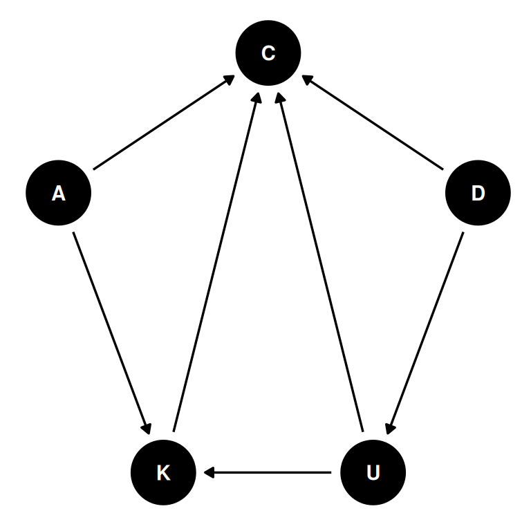
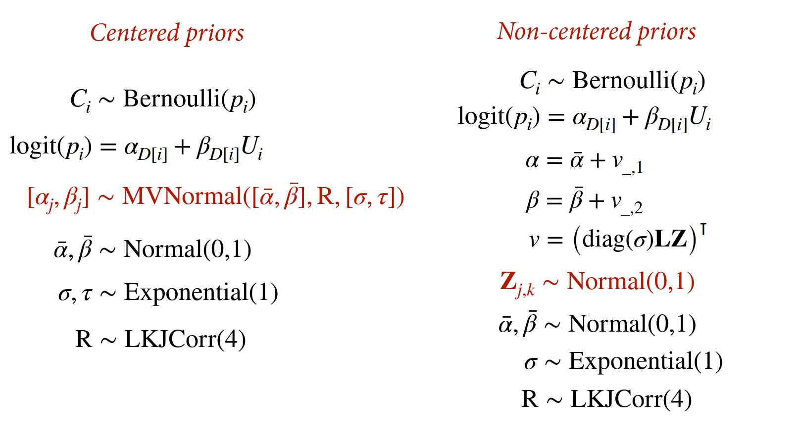
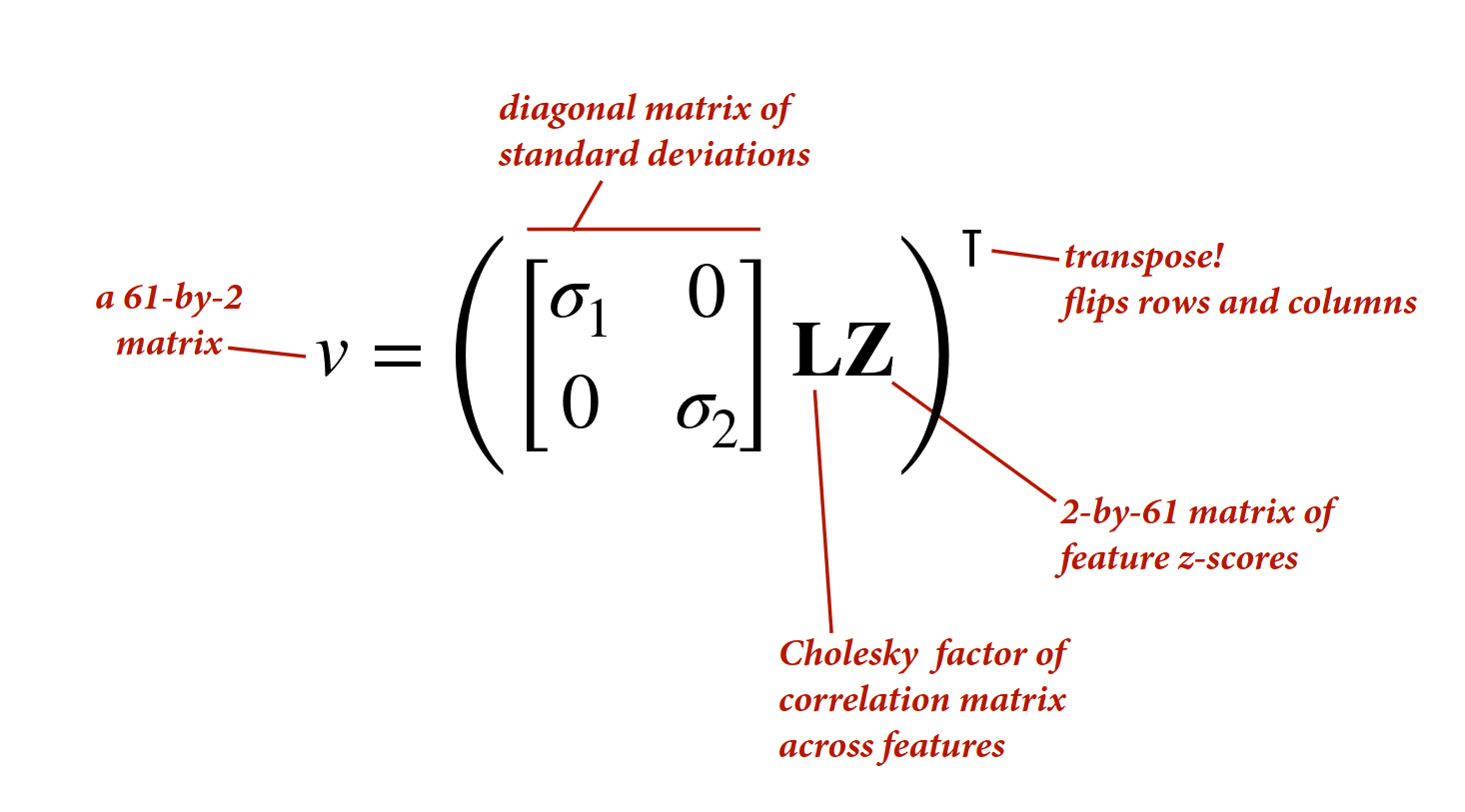
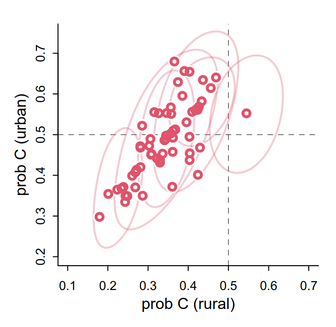
There is useful information to transfer across features, here we note there is a correlation between rural and urban probability of use within districts. A model that uses two 1-dimensional distributions (intercepts and slopes) does not consider the covariance structure between rural and urban within district.

Comparing the centered and non-centered model specification for the model using the multivariate normal specification with correlated features.

Simulating a synthetic dataset for this kind of complex system is challenging and is likely best done with more detailed tools than eg. expecting a linear responses, instead with eg. an agent based model.

Divergent transitions

Because of high curvature, the physics simulation runs off the surface. One option is to choose a smaller step size, but this results in much longer sampling time. Alternatively, re-express the “centered” model as a “non-centered” model.