Introduction to camtrapmonitoring

The {camtrapmonitoring} package provides functions for planning and evaluating camera trap surveys. The recommended approach is to first sample a set of candidate camera trap locations larger than the intended number of locations. Next, these candidate locations are evaluated using spatial layers to measure their deployment feasibility (such as distance to road) and to quantify their bias and coverage of project-specific characteristics (such as distribution across specific land cover classes).

{camtrapmonitoring} is designed to work with modern spatial R packages: {sf} and {terra}.

library(camtrapmonitoring)
library(sf)
#> Linking to GEOS 3.10.2, GDAL 3.4.1, PROJ 8.2.1; sf_use_s2() is TRUE
library(terra)
#> terra 1.7.65

Sampling candidate camera trap locations

The sample_ct function returns candidate camera trap locations using sf::st_sample across the user’s region of interest. Options include “regular”, “random” or “hexagonal” sampling across the entire region of interest or stratified by a column in the provided features.

The example data “clearwater_lake_density” is a simulated species density grid near Clearwater Lake, Manitoba. It is a simple feature collection of polygons with a column named “density” (High, Medium, Low).

We will randomly sample candidate camera trap locations, stratified by the simulated species density.

data("clearwater_lake_density")

plot(clearwater_lake_density, key.width = lcm(5))


pts <- sample_ct(
    region = clearwater_lake_density, 
    n = 25, 
    type = 'random', 
    strata = 'density'
)

plot(pts)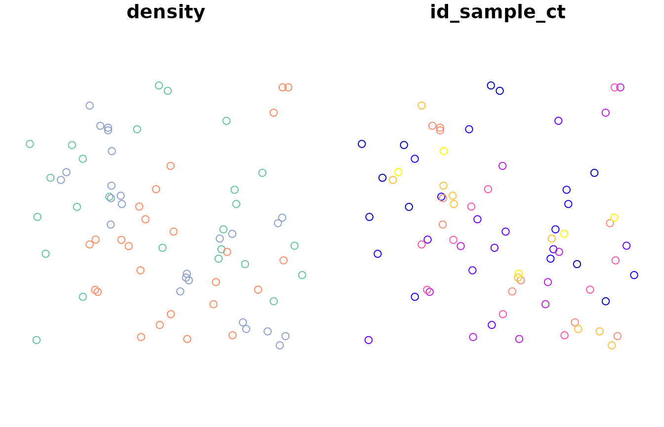

Evaluating candidate camera trap locations

To evaluate candidate camera trap locations, determine each spatial layer required and the criteria associated with it. For example:

Deployment feasibility

elevation
- point sample
- buffered point sample
roads
- distance to

Characteristics of candidate locations

land cover
- point sample
hydrology
- distance to
wetlands
- distance to

Deployment feasibility

First, we will evaluate the deployment feasibility layers. Note the example elevation data is an external TIF file that can be loaded with the {terra} package.

The eval_* family of functions return a vector of values for each candidate camera trap location. These vectors can be added to the simple features objects using the base R df$name <- value syntax (shown here) or with dplyr::mutate. eval_* functions take ‘features’ (candidate camera trap locations) and a ‘target’ covariate to evaluate each candidate location with. For eval_pt and eval_buffer, ‘target’ covariates are expected to be raster layers while eval_dist expects a ‘target’ vector object.

# Load data
clearwater_lake_elevation_path <- system.file('extdata', 'clearwater_lake_elevation.tif', package = 'camtrapmonitoring')
clearwater_lake_elevation <- rast(clearwater_lake_elevation_path)

data("clearwater_lake_roads")



# Evaluate elevation using point sample
pts$elev_pt <- eval_pt(features = pts, target = clearwater_lake_elevation)

# Evaluate elevation using buffered point sample
pts$elev_buffer_1e3 <- eval_buffer(
    features = pts, 
    target = clearwater_lake_elevation,
    buffer_size = 1e3
)

# Evaluate distance to roads
pts$road_dist <- eval_dist(features = pts, target = clearwater_lake_roads)



# Plot results
plot(pts)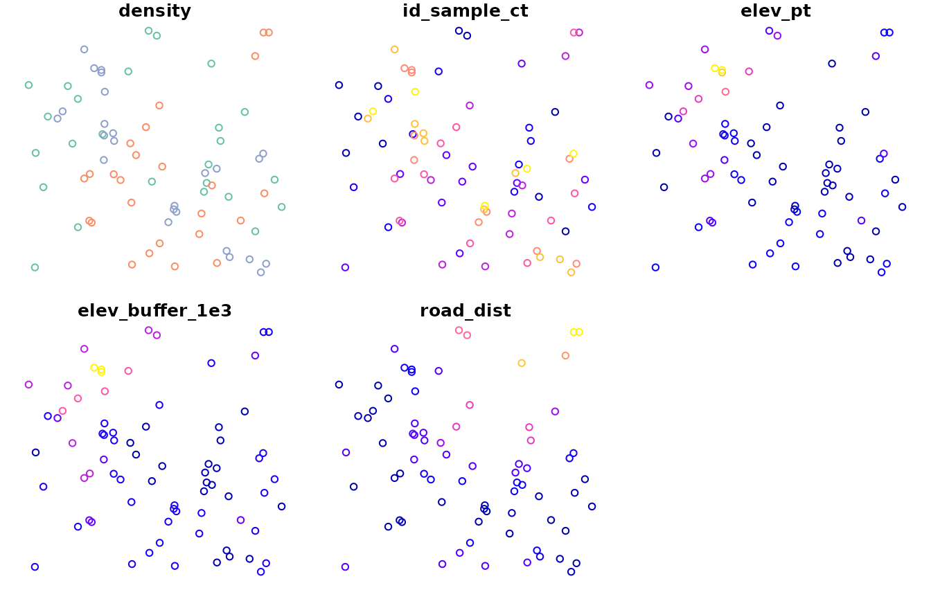

Characteristics of candidate locations

Next, we will evaluate the characteristics of candidate locations. Note the example land cover data is an external TIF file that can be loaded with the {terra} package.

# Load data
clearwater_lake_land_cover_path <- system.file('extdata', 'clearwater_lake_land_cover.tif', package = 'camtrapmonitoring')
clearwater_lake_land_cover <- rast(clearwater_lake_land_cover_path)

data("clearwater_lake_hydro")
data("clearwater_lake_wetlands")



# Evaluate land cover using point sample
pts$lc_pt <- eval_pt(features = pts, target = clearwater_lake_land_cover)

# Evaluate distance to hydrology
pts$hydro_dist <- eval_dist(features = pts, target = clearwater_lake_hydro)

# Evaluate distance to wetland
pts$wetland_dist <- eval_dist(features = pts, target = clearwater_lake_wetlands)



# Plot results
plot(pts)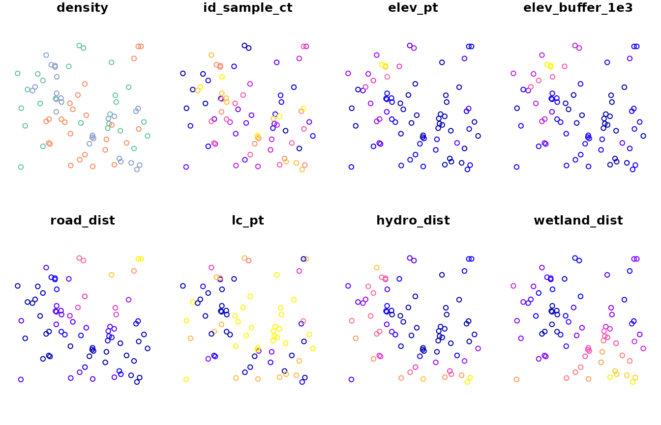

Selection from candidate camera trap locations

To select camera trap locations, define the criteria for selecting and sorting candidate locations.

Criteria for selection:

Maximum distance from roads: 3000 m
Maximum elevation: 300 m
Select only forest land cover classes: 1, 2, 5, 6

Criteria for sorting:

Nearer to wetlands
Farther from major lakes

# Selection criteria
max_road_dist_m <- 3000
max_elev_m <- 300
ls_lc_classes <- c(1, 2, 5, 6)

# Select out of candidate points
select_pts <- pts[pts$road_dist < max_road_dist_m &
                                        pts$elev_pt < max_elev_m &
                                        pts$lc_pt %in% ls_lc_classes,]

plot(select_pts)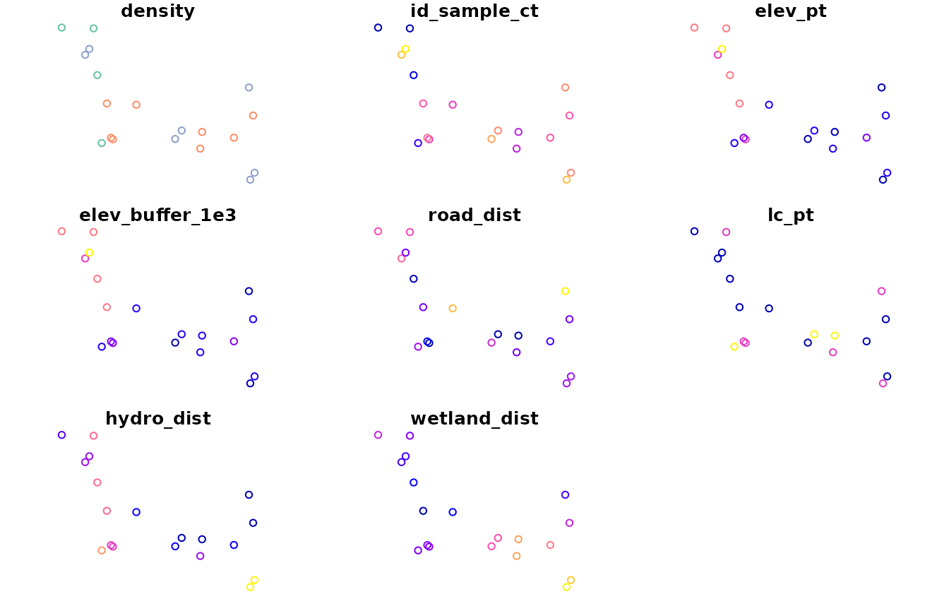

# Sorting criteria
ordered <- order(select_pts$wetland_dist, -select_pts$hydro_dist)

order_select_pts <- select_pts[ordered,]
print(order_select_pts)
#> Simple feature collection with 19 features and 8 fields
#> Geometry type: POINT
#> Dimension:     XY
#> Bounding box:  xmin: 345435.6 ymin: 5975880 xmax: 374851.2 ymax: 6002167
#> Projected CRS: WGS 84 / UTM zone 14N
#> First 10 features:
#>    density                 geometry id_sample_ct elev_pt elev_buffer_1e3
#> 26  Medium   POINT (355178 5987488)           26     270        268.4948
#> 29  Medium POINT (349973.9 5990861)           29     285        283.7429
#> 65     Low POINT (354187.8 5998225)           65     288        289.7754
#> 34  Medium POINT (352093.7 5985170)           34     277        277.4647
#> 61     Low POINT (374131.2 5989910)           61     261        263.2495
#> 28  Medium POINT (356921.1 5984658)           28     261        261.5417
#> 16    High POINT (347104.1 5996177)           16     269        273.1169
#> 30  Medium POINT (346239.8 5988300)           30     260        261.7837
#> 46  Medium POINT (357788.5 5982133)           46     267        265.1705
#> 5     High POINT (354050.3 5980438)            5     275        276.2097
#>     road_dist lc_pt hydro_dist wetland_dist
#> 26 2774.07058     1 1861.46668     1960.820
#> 29  972.79303     1 5797.01559     2246.728
#> 65 2659.74974     1 2118.18358     2269.173
#> 34 1391.05592     1 4439.60697     3517.056
#> 61 2529.17964     6   92.59484     4200.977
#> 28   81.18676     1  130.02211     5154.464
#> 16 1030.59514     1 2529.62768     5479.958
#> 30 2376.91611     5 7874.03421     6432.827
#> 46  263.79756     6  763.74124     7690.023
#> 5  1747.04087     1 3453.34390     8081.887

Establishing camera trap grids

The function grid_ct allows the user to establish sampling grids around focal locations selected above. The grid_design function is provided to the user to help explore grid layout options, using either the ‘case’ argument or the ‘n’ argument.

plot(grid_design(distance = 100, case = 'queen'))


plot(grid_design(distance = 100, case = 'bishop'))


plot(grid_design(distance = 100, case = 'rook'))


plot(grid_design(distance = 100, case = 'triplet'))


plot(grid_design(distance = 250, n = 13))

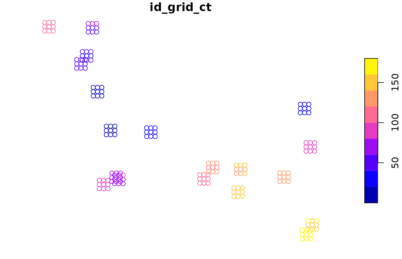
After the grid design is selected, the grid_ct function can be used with the selected camera trap locations.

ct_grids <- grid_ct(
    features = order_select_pts,
    distance = 500,
    case = 'queen'
)

plot(ct_grids['id_grid_ct'][1])

Example data sources

Example data used in the {camtrapmonitoring} package come from open data sources we gratefully acknowledge in the help page for each data set. Also see the “data-raw” directory in the package source for full data preprocessing steps.

Alec L. Robitaille

2024-01-27

Sampling candidate camera trap locations

Evaluating candidate camera trap locations

Deployment feasibility

Characteristics of candidate locations

Selection from candidate camera trap locations

Establishing camera trap grids

Example data sources